基于趋势和季节性的时间序列预测

时间序列预测是基于时间数据进行预测的任务。它包括建立模型来进行观测，并在诸如天气、工程、经济、金融或商业预测等应用中推动未来的决策。

本文主要介绍时间序列预测并描述任何时间序列的两种主要模式(趋势和季节性)。并基于这些模式对时间序列进行分解。最后使用一个被称为Holt-Winters季节方法的预测模型，来预测有趋势和/或季节成分的时间序列数据。

为了涵盖所有这些内容，我们将使用一个时间序列数据集，包括1981年至1991年期间墨尔本(澳大利亚)的温度。这个数据集可以从这个Kaggle下载，也可以本文最后的GitHub下载，其中包含本文的数据和代码。该数据集由澳大利亚政府气象局托管，并根据该局的“默认使用条款”(Open Access Licence)获得许可。

导入库和数据

首先，导入运行代码所需的下列库。除了最典型的库之外，该代码还基于statsmomodels库提供的函数，该库提供了用于估计许多不同统计模型的类和函数，如统计测试和预测模型。

from datetime import datetime, timedelta
import matplotlib.pyplot as plt
import numpy as np
import pandas as pd
import statsmodels.api as sm
from statsmodels.tsa.stattools import adfuller, kpss
from statsmodels.tsa.api import ExponentialSmoothing
%matplotlib inline

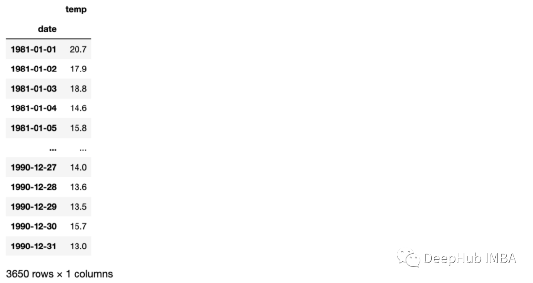
下面是导入数据的代码。数据由两列组成，一列是日期，另一列是1981年至1991年间墨尔本(澳大利亚)的温度。

# date
numdays = 365*10 + 2
base = '2010-01-01'
base = datetime.strptime(base, '%Y-%m-%d')
date_list = [base + timedelta(days=x) for x in range(numdays)]
date_list = np.array(date_list)
print(len(date_list), date_list[0], date_list[-1])

# temp
x = np.linspace(-np.pi, np.pi, 365)
temp_year = (np.sin(x) + 1.0) * 15
x = np.linspace(-np.pi, np.pi, 366)
temp_leap_year = (np.sin(x) + 1.0)
temp_s = []
for i in range(2010, 2020):
    if i == 2010:
        temp_s = temp_year + np.random.rand(365) * 20
    elif i in [2012, 2016]:
        temp_s = np.concatenate((temp_s, temp_leap_year * 15 + np.random.rand(366) * 20 + i % 2010))
    else:
        temp_s = np.concatenate((temp_s, temp_year + np.random.rand(365) * 20 + i % 2010))
print(len(temp_s))

# df
data = np.concatenate((date_list.reshape(-1, 1), temp_s.reshape(-1, 1)), axis=1)
df_orig = pd.DataFrame(data, columns=['date', 'temp'])
df_orig['date'] =  pd.to_datetime(df_orig['date'], format='%Y-%m-%d')
df = df_orig.set_index('date')
df.sort_index(inplace=True)
df

可视化数据集

在我们开始分析时间序列的模式之前，让我们将每个垂直虚线对应于一年开始的数据可视化。

ax = df_orig.plot(x='date', y='temp', figsize=(12,6))
xcoords = ['2010-01-01', '2011-01-01', '2012-01-01', '2013-01-01', '2014-01-01',
           '2015-01-01', '2016-01-01', '2017-01-01', '2018-01-01', '2019-01-01']
for xc in xcoords:
    plt.axvline(x=xc, color='black', linestyle='--')
ax.set_ylabel('temperature')

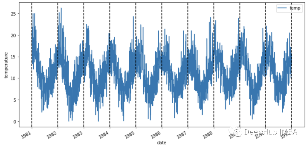
在进入下一节之前，让我们花点时间看一下数据。这些数据似乎有一个季节性的变化，冬季温度上升，夏季温度下降(南半球)。而且气温似乎不会随着时间的推移而增加，因为无论哪一年的平均气温都是相同的。

时间序列模式

时间序列预测模型使用数学方程(s)在一系列历史数据中找到模式。然后使用这些方程将数据[中的历史时间模式投射到未来。

有四种类型的时间序列模式:

趋势:数据的长期增减。趋势可以是任何函数，如线性或指数，并可以随时间改变方向。

季节性:以固定的频率(一天中的小时、星期、月、年等)在系列中重复的周期。季节模式存在一个固定的已知周期

周期性:当数据涨跌时发生，但没有固定的频率和持续时间，例如由经济状况引起。

噪音:系列中的随机变化。

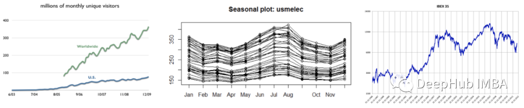
大多数时间序列数据将包含一个或多个模式，但可能不是全部。这里有一些例子，我们可以识别这些时间序列模式:

维基百科年度受众(左图):在这张图中，我们可以确定一个增加的趋势，受众每年线性增加。

美国用电量季节性图(中图):每条线对应的是一年，因此我们可以观察到每年的用电量重复出现的季节性。

ibex35的日收盘价(右图):这个时间序列随着时间的推移有一个增加的趋势，以及一个周期性的模式，因为有一些时期ibex35由于经济原因而下降。

如果我们假设对这些模式进行加法分解，我们可以这样写:

Y[t] = t [t] + S[t] + e[t]

其中Y[t]为数据，t [t]为趋势周期分量，S[t]为季节分量，e[t]为噪声，t为时间周期。

另一方面，乘法分解可以写成:

Y[t] = t [t] *S[t] *e[t]

当季节波动不随时间序列水平变化时，加法分解是最合适的方法。相反，当季节成分的变化与时间序列水平成正比时，则采用乘法分解更为合适。

分解数据

平稳时间序列被定义为其不依赖于观察到该序列的时间。因此具有趋势或季节性的时间序列不是平稳的，而白噪声序列是平稳的。从数学意义上讲，如果一个时间序列的均值和方差不变，且协方差与时间无关，那么这个时间序列就是平稳的。有不同的例子来比较平稳和非平稳时间序列。一般来说，平稳时间序列不会有长期可预测的模式。

为什么稳定性很重要呢?

平稳性已经成为时间序列分析中许多实践和工具的常见假设。其中包括趋势估计、预测和因果推断等。因此，在许多情况下，需要确定数据是否是由固定过程生成的，并将其转换为具有该过程生成的样本的属性。

如何检验时间序列的平稳性呢?

我们可以用两种方法来检验。一方面，我们可以通过检查时间序列的均值和方差来手动检查。另一方面，我们可以使用测试函数来评估平稳性。

有些情况可能会让人感到困惑。例如一个没有趋势和季节性但具有周期行为的时间序列是平稳的，因为周期的长度不是固定的。

查看趋势

为了分析时间序列的趋势，我们首先使用有30天窗口的滚动均值方法分析随时间推移的平均值。

def analyze_stationarity(timeseries, title):
    fig, ax = plt.subplots(2, 1, figsize=(16, 8))

    rolmean = pd.Series(timeseries).rolling(window=30).mean() 
    rolstd = pd.Series(timeseries).rolling(window=30).std()
    ax[0].plot(timeseries, label= title)
    ax[0].plot(rolmean, label='rolling mean');
    ax[0].plot(rolstd, label='rolling std (x10)');
    ax[0].set_title('30-day window')
    ax[0].legend()
    
    rolmean = pd.Series(timeseries).rolling(window=365).mean() 
    rolstd = pd.Series(timeseries).rolling(window=365).std()
    ax[1].plot(timeseries, label= title)
    ax[1].plot(rolmean, label='rolling mean');
    ax[1].plot(rolstd, label='rolling std (x10)');
    ax[1].set_title('365-day window')
    
pd.options.display.float_format = '{:.8f}'.format
analyze_stationarity(df['temp'], 'raw data')
    ax[1].legend()

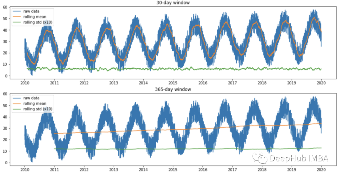
在上图中，我们可以看到使用30天窗口时滚动均值是如何随时间波动的，这是由数据的季节性模式引起的。此外，当使用365天窗口时，滚动平均值随时间增加，表明随时间略有增加的趋势。

这也可以通过一些测试来评估，如Dickey-Fuller (ADF)和Kwiatkowski, Phillips, Schmidt和Shin (KPSS):

ADF检验的结果(p值低于0.05)表明，存在的原假设可以在95%的置信水平上被拒绝。因此，如果p值低于0.05，则时间序列是平稳的。

def ADF_test(timeseries):
    print("Results of Dickey-Fuller Test:")
    dftest = adfuller(timeseries, autolag="AIC")
    dfoutput = pd.Series(
        dftest[0:4],
        index=[
            "Test Statistic",
            "p-value",
            "Lags Used",
            "Number of Observations Used",
        ],
    )
    for key, value in dftest[4].items():
        dfoutput["Critical Value (%s)" % key] = value
    print(dfoutput)

ADF_test(df)

Results of Dickey-Fuller Test:
Test Statistic                  -3.69171446
p-value                          0.00423122
Lags Used                       30.00000000
Number of Observations Used   3621.00000000
Critical Value (1%)             -3.43215722
Critical Value (5%)             -2.86233853
Critical Value (10%)            -2.56719507
dtype: float64

KPSS检验的结果(p值高于0.05)表明，在95%的置信水平下，不能拒绝的零假设。因此如果p值低于0.05，则时间序列不是平稳的。

def KPSS_test(timeseries):
    print("Results of KPSS Test:")
    kpsstest = kpss(timeseries.dropna(), regression="c", nlags="auto")    
    kpss_output = pd.Series(
        kpsstest[0:3], index=["Test Statistic", "p-value", "Lags Used"]
    )
    for key, value in kpsstest[3].items():
        kpss_output["Critical Value (%s)" % key] = value
    print(kpss_output)

KPSS_test(df)

Results of KPSS Test:
Test Statistic           1.04843270
p-value                  0.01000000
Lags Used               37.00000000
Critical Value (10%)     0.34700000
Critical Value (5%)      0.46300000
Critical Value (2.5%)    0.57400000
Critical Value (1%)      0.73900000
dtype: float64

虽然这些检验似乎是为了检查数据的平稳性，但这些检验对于分析时间序列的趋势而不是季节性是有用的。

统计结果还显示了时间序列的平稳性的影响。虽然两个检验的零假设是相反的。ADF检验表明时间序列是平稳的(p值> 0.05)，而KPSS检验表明时间序列不是平稳的(p值> 0.05)。但这个数据集创建时带有轻微的趋势，因此结果表明，KPSS测试对于分析这个数据集更准确。

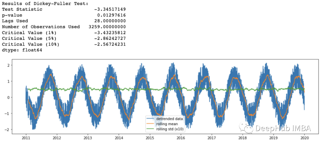
为了减少数据集的趋势，我们可以使用以下方法消除趋势:

df_detrend = (df - df.rolling(window=365).mean()) / df.rolling(window=365).std()

analyze_stationarity(df_detrend['temp'].dropna(), 'detrended data')
ADF_test(df_detrend.dropna())

检查季节性

正如在之前从滑动窗口中观察到的，在我们的时间序列中有一个季节模式。因此应该采用差分方法来去除时间序列中潜在的季节或周期模式。由于样本数据集具有12个月的季节性，我使用了365个滞后差值:

df_365lag =  df - df.shift(365)

analyze_stationarity(df_365lag['temp'].dropna(), '12 lag differenced data')
ADF_test(df_365lag.dropna())

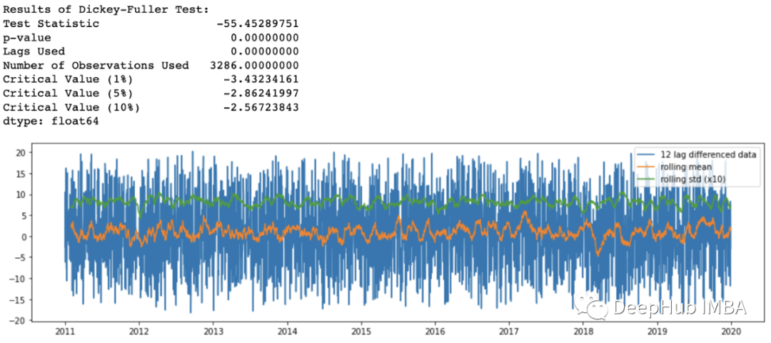
现在，滑动均值和标准差随着时间的推移或多或少保持不变，所以我们有一个平稳的时间序列。

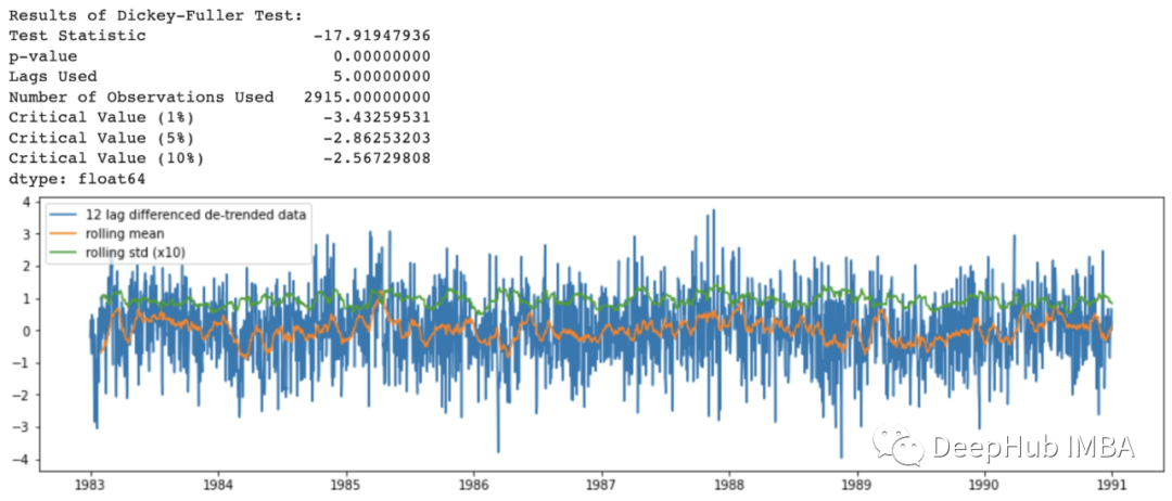
上面方法合在一起的代码如下：

df_365lag_detrend =  df_detrend - df_detrend.shift(365)

analyze_stationarity(df_365lag_detrend['temp'].dropna(), '12 lag differenced de-trended data')
ADF_test(df_365lag_detrend.dropna())

分解模式

基于上述模式的分解可以通过' statmodels '包中的一个有用的Python函数seasonal_decomposition来实现:

def seasonal_decompose (df):
    decomposition = sm.tsa.seasonal_decompose(df, model='additive', freq=365)

    trend = decomposition.trend
    seasonal = decomposition.seasonal
    residual = decomposition.resid

    fig = decomposition.plot()
    fig.set_size_inches(14, 7)
    plt.show()

    return trend, seasonal, residual

seasonal_decompose(df)

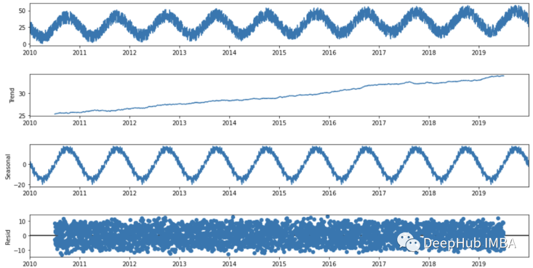
在看了分解图的四个部分后，可以说，在我们的时间序列中有很强的年度季节性成分，以及随时间推移的增加趋势模式。

时序建模

时间序列数据的适当模型将取决于数据的特定特征，例如，数据集是否具有总体趋势或季节性。请务必选择最适数据的模型。

我们可以使用下面这些模型：

Autoregression (AR)
Moving Average (MA)
Autoregressive Moving Average (ARMA)
Autoregressive Integrated Moving Average (ARIMA)
Seasonal Autoregressive Integrated Moving-Average (SARIMA)
Seasonal Autoregressive Integrated Moving-Average with Exogenous Regressors (SARIMAX)
Vector Autoregression (VAR)
Vector Autoregression Moving-Average (VARMA)
Vector Autoregression Moving-Average with Exogenous Regressors (VARMAX)
Simple Exponential Smoothing (SES)
Holt Winter’s Exponential Smoothing (HWES)

由于我们的数据中存在季节性，因此选择HWES，因为它适用于具有趋势和/或季节成分的时间序列数据。

这种方法使用指数平滑来编码大量的过去的值，并使用它们来预测现在和未来的“典型”值。指数平滑指的是使用指数加权移动平均(EWMA)“平滑”一个时间序列。

在实现它之前，让我们创建训练和测试数据集:

y = df['temp'].astype(float)
y_to_train = y[:'2017-12-31']
y_to_val = y['2018-01-01':]
predict_date = len(y) - len(y[:'2017-12-31'])

下面是使用均方根误差(RMSE)作为评估模型误差的度量的实现。

def holt_win_sea(y, y_to_train, y_to_test, seasonal_period, predict_date):

    fit1 = ExponentialSmoothing(y_to_train, seasonal_periods=seasonal_period, trend='add', seasonal='add').fit(use_boxcox=True)
    fcast1 = fit1.forecast(predict_date).rename('Additive')
    mse1 = ((fcast1 - y_to_test.values) ** 2).mean()
    print('The Root Mean Squared Error of additive trend, additive seasonal of '+ 
          'period season_length={} and a Box-Cox transformation {}'.format(seasonal_period,round(np.sqrt(mse1), 2)))

    y.plot(marker='o', color='black', legend=True, figsize=(10, 5))
    fit1.fittedvalues.plot(style='--', color='red', label='train')
    fcast1.plot(style='--', color='green', label='test')
    plt.ylabel('temp')
    plt.title('Additive trend and seasonal')
    plt.legend()
    plt.show()

holt_win_sea(y, y_to_train, y_to_val, 365, predict_date)

The Root Mean Squared Error of additive trend, additive seasonal of period season_length=365 and a Box-Cox transformation 6.27

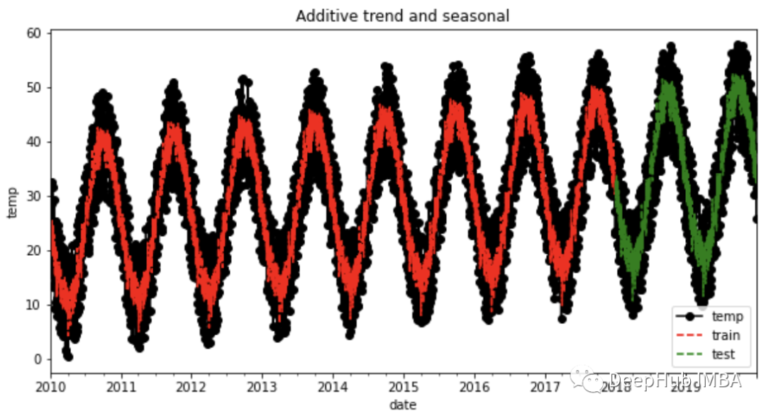
从图中我们可以观察到模型是如何捕捉时间序列的季节性和趋势的，在异常值的预测上则存在一些误差。

总结

在本文中，我们通过一个基于温度数据集的实际示例来介绍趋势和季节性。除了检查趋势和季节性之外，我们还看到了如何降低它，以及如何创建一个基本模型，利用这些模式来推断未来几天的温度。

了解主要的时间序列模式和学习如何实现时间序列预测模型是至关重要的，因为它们有许多应用。

本文数据和代码：

https://github.com/javiferfer/medium/blob/master/time_series_forecast/modeling_synthetic_dataset.ipynb

作者：Javier Fernandez

标签：机器学习数据分析时间序列

基于趋势和季节性的时间序列预测

导入库和数据

可视化数据集

时间序列模式

分解数据

时序建模

总结

发表评论

“基于趋势和季节性的时间序列预测”的评论:

关于作者

Deephub

相关阅读

文章导航