余弦相似度算法进行客户流失分类预测

余弦相似性是一种用于计算两个向量之间相似度的方法，常被用于文本分类和信息检索领域。具体来说，假设有两个向量A和B，它们的余弦相似度可以通过以下公式计算：

其中，dot_product(A, B)表示向量A和B的点积，norm(A)和norm(B)分别表示向量A和B的范数。如果A和B越相似，它们的余弦相似度就越接近1，反之亦然。

数据集

我们这里用的演示数据集来自一个datacamp：

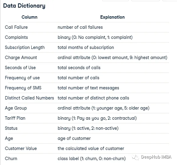
这个数据集来自一家伊朗电信公司，每一行代表一个客户一年的时间。除了客户流失标签，还有客户活动的信息，比如呼叫失败和订阅时长等等。我们最后要预测的是这个客户是否流失，也就是一个二元分类的问题。

数据集如下：

 import pandas as pd
 df = pd.read_csv("data/customer_churn.csv")
 

我们先区分训练和验证集：

 from sklearn.model_selection import train_test_split
 
 # split the dataframe into 70% training and 30% testing sets
 train_df, test_df = train_test_split(df, test_size=0.3)

SVM

为了进行对比，我们先使用SVM做一个基础模型

 fromsklearn.svmimportSVC
 fromsklearn.metricsimportclassification_report, confusion_matrix
 
 # define the range of C and gamma values to try
 c_values= [0.1, 1, 10, 100]
 gamma_values= [0.1, 1, 10, 100]
 
 # initialize variables to store the best result
 best_accuracy=0
 best_c=None
 best_gamma=None
 best_predictions=None
 
 # loop over the different combinations of C and gamma values
 forcinc_values:
     forgammaingamma_values:
         # initialize the SVM classifier with RBF kernel, C, and gamma
         clf=SVC(kernel='rbf', C=c, gamma=gamma, random_state=42)
 
         # fit the classifier on the training set
         clf.fit(train_df.drop('Churn', axis=1), train_df['Churn'])
 
         # predict the target variable of the test set
         y_pred=clf.predict(test_df.drop('Churn', axis=1))
 
         # calculate accuracy and store the result if it's the best so far
         accuracy=clf.score(test_df.drop('Churn', axis=1), test_df['Churn'])
         ifaccuracy>best_accuracy:
             best_accuracy=accuracy
             best_c=c
             best_gamma=gamma
             best_predictions=y_pred
 
 # print the best result and the confusion matrix
 print(f"Best result: C={best_c}, gamma={best_gamma}, accuracy={best_accuracy:.2f}")
 print("Confusion matrix:")
 print(confusion_matrix(test_df['Churn'], best_predictions))

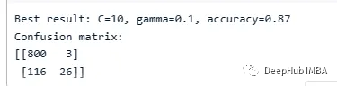
可以看到支持向量机得到了87%的准确率，并且很好地预测了客户流失。

余弦相似度算法

这段代码使用训练数据集来计算类之间的余弦相似度。

 importpandasaspd
 fromsklearn.metrics.pairwiseimportcosine_similarity
 
 # calculate the cosine similarity matrix between all rows of the dataframe
 cosine_sim=cosine_similarity(train_df.drop('Churn', axis=1))
 
 # create a dataframe from the cosine similarity matrix
 cosine_sim_df=pd.DataFrame(cosine_sim, index=train_df.index, columns=train_df.index)
 
 # create a copy of the train_df dataframe without the churn column
 train_df_no_churn=train_df.drop('Churn', axis=1)
 
 # calculate the mean cosine similarity for class 0 vs. class 0
 class0_cosine_sim_0=cosine_sim_df.loc[train_df[train_df['Churn'] ==0].index, train_df[train_df['Churn'] ==0].index].mean().mean()
 
 # calculate the mean cosine similarity for class 0 vs. class 1
 class0_cosine_sim_1=cosine_sim_df.loc[train_df[train_df['Churn'] ==0].index, train_df[train_df['Churn'] ==1].index].mean().mean()
 
 # calculate the mean cosine similarity for class 1 vs. class 1
 class1_cosine_sim_1=cosine_sim_df.loc[train_df[train_df['Churn'] ==1].index, train_df[train_df['Churn'] ==1].index].mean().mean()
 
 # display the mean cosine similarities for each pair of classes
 print('Mean cosine similarity (class 0 vs. class 0):', class0_cosine_sim_0)
 print('Mean cosine similarity (class 0 vs. class 1):', class0_cosine_sim_1)
 print('Mean cosine similarity (class 1 vs. class 1):', class1_cosine_sim_1)

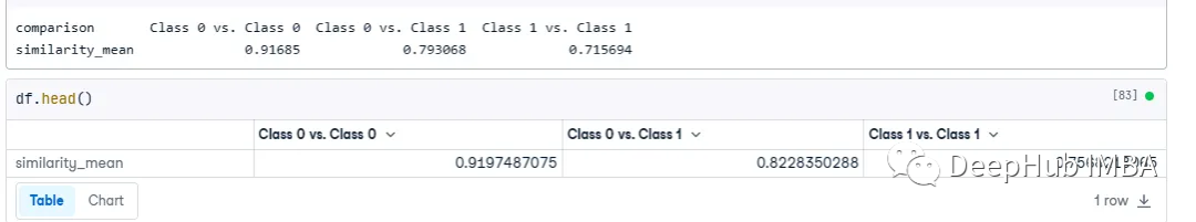
下面是它们的余弦相似度:

然后我们生成一个DF

 importpandasaspd
 
 # create a dictionary with the mean and standard deviation values for each comparison
 data= {
     'comparison': ['Class 0 vs. Class 0', 'Class 0 vs. Class 1', 'Class 1 vs. Class 1'],
     'similarity_mean': [class0_cosine_sim_0, class0_cosine_sim_1, class1_cosine_sim_1],
 }
 
 # create a Pandas DataFrame from the dictionary
 df=pd.DataFrame(data)
 
 df=df.set_index('comparison').T
 
 
 # print the resulting DataFrame
 print(df)

下面就是把这个算法应用到训练数据集上。我取在训练集上创建一个sample_churn_0，其中包含10个样本以的距离。

 # create a DataFrame containing a random sample of 10 points where Churn is 0
 sample_churn_0=train_df[train_df['Churn'] ==0].sample(n=10)

然后将它交叉连接到test_df。这将使test_df扩充为10倍的行数，因为每个测试记录的右侧有10个示例记录。

 importpandasaspd
 
 # assume test_df and sample_churn_0 are your dataframes
 
 # add a column to both dataframes with a common value to join on
 test_df['join_col'] =1
 sample_churn_0['join_col'] =1
 
 # perform the cross-join using merge()
 result_df=pd.merge(test_df, sample_churn_0, on='join_col')
 
 # drop the join_col column from the result dataframe
 result_df=result_df.drop('join_col', axis=1)

现在我们对交叉连接DF的左侧和右侧进行余弦相似性比较。

 importpandasaspd
 fromsklearn.metrics.pairwiseimportcosine_similarity
 
 # Extract the "_x" and "_y" columns from the result_df DataFrame, excluding the "Churn_x" and "Churn_y" columns
 df_x=result_df[[colforcolinresult_df.columnsifcol.endswith('_x') andnotcol.startswith('Churn_')]]
 df_y=result_df[[colforcolinresult_df.columnsifcol.endswith('_y') andnotcol.startswith('Churn_')]]
 
 # Calculate the cosine similarities between the two sets of vectors on each row
 cosine_sims= []
 foriinrange(len(df_x)):
     cos_sim=cosine_similarity([df_x.iloc[i]], [df_y.iloc[i]])[0][0]
     cosine_sims.append(cos_sim)
 
 # Add the cosine similarity values as a new column in the result_df DataFrame
 result_df['cos_sim'] =cosine_sims

然后用下面的代码提取所有的列名:

 x_col_names = [col for col in result_df.columns if col.endswith('_x')]

这样我们就可以进行分组并获得每个test_df记录的平均余弦相似度(目前重复10次)，然后在grouped_df中，我们将其重命名为x_col_names:

 grouped_df = result_df.groupby(result_df.columns[:14].tolist()).agg({'cos_sim': 'mean'})
 
 grouped_df = grouped_df.rename_axis(x_col_names).reset_index()
 
 grouped_df.head()

最后我们计算这10个样本的平均余弦相似度。

在上面步骤中，我们计算的分类相似度的df是这个：

我们就使用这个数值作为分类的参考。首先，我们需要将其交叉连接到grouped_df(与test_df相同，但具有平均余弦相似度):

 cross_df = grouped_df.merge(df, how='cross')
 cross_df = cross_df.iloc[:, :-1]

结果如下：

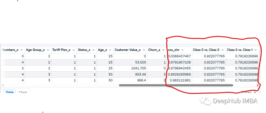
最后我们得到了3列：Class 0 vs. Class 0, and Class 0 vs. Class 1，然后我们需要得到类之间的差别：

 cross_df['diff_0'] = abs(cross_df['cos_sim'] - df['Class 0 vs. Class 0'].iloc[0])
 cross_df['diff_1'] = abs(cross_df['cos_sim'] - df['Class 0 vs. Class 1'].iloc[0])

预测的代码如下：

 # Add a new column 'predicted_churn'
 cross_df['predicted_churn'] = ''
 
 # Loop through each row and check the minimum difference
 for idx, row in cross_df.iterrows():
     if row['diff_0'] < row['diff_1']:
         cross_df.at[idx, 'predicted_churn'] = 0
     else:
         cross_df.at[idx, 'predicted_churn'] = 1

最后我们看看结果：

 grouped_df__2 = cross_df.groupby(['predicted_churn', 'Churn_x']).size().reset_index(name='count')
 grouped_df__2['percentage'] = grouped_df__2['count'] / grouped_df__2['count'].sum() * 100
 
 grouped_df__2.head()

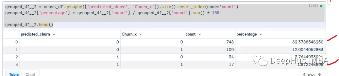
可以看到，模型的准确率为84.25%。但是我们可以看到，他的混淆矩阵看到对于某些预测要比svm好，也就是说它可以在一定程度上解决类别不平衡的问题。

总结

余弦相似性本身并不能直接解决类别不平衡的问题，因为它只是一种计算相似度的方法，而不是一个分类器。但是，余弦相似性可以作为特征表示方法，来提高类别不平衡数据集的分类性能。本文只是作为一个样例还有可以提高的空间。

本文的数据集在这里：（需要注册）

https://www.datacamp.com/workspace/datasets/dataset-r-telecom-customer-churn

如果你有兴趣可以自行尝试。

作者：Ashutosh Malgaonkar

x