评估和选择最佳学习模型的一些指标总结

在评估模型时，虽然准确性是训练阶段模型评估和应用模型调整的重要指标，但它并不是模型评估的最佳指标，我们可以使用几个评估指标来评估我们的模型。

因为我们用于构建大多数模型的数据是不平衡的，并且在对数据进行训练时模型可能会过拟合。在本文中，我将讨论和解释其中的一些方法，并给出使用 Python 代码的示例。

混淆矩阵

对于分类模型使用混淆矩阵是一个非常好的方法来评估我们的模型。它对于可视化的理解预测结果是非常有用的，因为正和负的测试样本的数量都会显示出来。并且它提供了有关模型如何解释预测的信息。混淆矩阵可用于二元和多项分类。它由四个矩阵组成：

#Import Libraries:
from random import random
from random import randint
import numpy as np
import pandas as pd
import matplotlib.pyplot as plt
import seaborn as sns
from sklearn.model_selection import train_test_split
from sklearn.linear_model import LogisticRegression
from sklearn.metrics import classification_report, confusion_matrix
from sklearn.metrics import precision_recall_curve
from sklearn.metrics import roc_curve

#Fabricating variables:
#Creating values for FeNO with 3 classes:
FeNO_0 = np.random.normal(15,20, 1000)
FeNO_1 = np.random.normal(35,20, 1000)
FeNO_2 = np.random.normal(65, 20, 1000)

#Creating values for FEV1 with 3 classes:
FEV1_0 = np.random.normal(4.50, 1, 1000)
FEV1_1 = np.random.uniform(3.75, 1.2, 1000)
FEV1_2 = np.random.uniform(2.35, 1.2, 1000)

#Creating values for Bronco Dilation with 3 classes:
BD_0 = np.random.normal(150,49, 1000)
BD_1 = np.random.uniform(250,50,1000)
BD_2 = np.random.uniform(350, 50, 1000)

#Creating labels variable with two classes (1)Disease (0)No disease:
no_disease = np.zeros((1500,), dtype=int)
disease = np.ones((1500,), dtype=int)

#Concatenate classes into one variable:
FeNO = np.concatenate([FeNO_0, FeNO_1, FeNO_2])
FEV1 = np.concatenate([FEV1_0, FEV1_1, FEV1_2])
BD = np.concatenate([BD_0, BD_1, BD_2])
dx = np.concatenate([not_asma, asma])

#Create DataFrame:
df = pd.DataFrame()#Add variables to DataFrame:
df['FeNO'] = FeNO.tolist()
df['FEV1'] = FEV1.tolist()
df['BD'] = BD.tolist()
df['dx'] = dx.tolist()

#Create X and y:
X = df.drop('dx', axis=1)
y = df['dx']#Train and Test split:
X_train, X_test, y_train, y_test = train_test_split(X, y, test_size=0.20)

#Build the model:
logisticregression = LogisticRegression().fit(X_train, y_train)

#Print accuracy metrics:
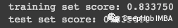
print("training set score: %f" % logisticregression.score(X_train, y_train))
print("test set score: %f" % logisticregression.score(X_test, y_test))

现在我们可以构建混淆矩阵并检查我们的模型了:

# Predicting labels from X_test data
y_pred = logisticregression.predict(X_test)

# Create the confusion matrix
confmx = confusion_matrix(y_test, y_pred)
f, ax = plt.subplots(figsize = (8,8))
sns.heatmap(confmx, annot=True, fmt='.1f', ax = ax)
plt.xlabel('Predicted Labels')
plt.ylabel('True Labels')
plt.title('Confusion Matrix')
plt.show();

可以看到，模型未能对42个标签[1]和57个标签[0]的进行分类。

上面的方法是二分类的情况，建立多分类的混淆矩阵的步骤是相似的。

#Fabricating variables:
#Creating values for FeNO with 3 classes:
FeNO_0 = np.random.normal(15,20, 1000)
FeNO_1 = np.random.normal(35,20, 1000)
FeNO_2 = np.random.normal(65, 20, 1000)

#Creating values for FEV1 with 3 classes:
FEV1_0 = np.random.normal(4.50, 1, 1000)
FEV1_1 = np.random.normal(3.75, 1.2, 1000)
FEV1_2 = np.random.normal(2.35, 1.2, 1000)

#Creating values for Broncho Dilation with 3 classes:
BD_0 = np.random.normal(150,49, 1000)
BD_1 = np.random.normal(250,50,1000)
BD_2 = np.random.normal(350, 50, 1000)

#Creating labels variable with three classes: 
no_disease = np.zeros((1000,), dtype=int)
possible_disease = np.ones((1000,), dtype=int)
disease = np.full((1000,), 2, dtype=int)

#Concatenate classes into one variable:
FeNO = np.concatenate([FeNO_0, FeNO_1, FeNO_2])
FEV1 = np.concatenate([FEV1_0, FEV1_1, FEV1_2])
BD = np.concatenate([BD_0, BD_1, BD_2])
dx = np.concatenate([no_disease, possible_disease, disease])

#Create DataFrame:
df = pd.DataFrame()

#Add variables to DataFrame:
df['FeNO'] = FeNO.tolist()
df['FEV1'] = FEV1.tolist()
df['BD'] = BD.tolist()
df['dx'] = dx.tolist()

#Creating X and y:
X = df.drop('dx', axis=1)
y = df['dx']#Data split into train and test:
X_train, X_test, y_train, y_test = train_test_split(X, y, test_size=0.20)#Fit Logistic Regression model:
logisticregression = LogisticRegression().fit(X_train, y_train)

#Evaluate Logistic Regression model:
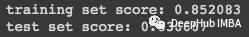
print("training set score: %f" % logisticregression.score(X_train, y_train))
print("test set score: %f" % logisticregression.score(X_test, y_test))

现在我们来创建混淆矩阵

# Predicting labels from X_test data
y_pred = logisticregression.predict(X_test)

# Create the confusion matrix
confmx = confusion_matrix(y_test, y_pred)
f, ax = plt.subplots(figsize = (8,8))
sns.heatmap(confmx, annot=True, fmt='.1f', ax = ax)
plt.xlabel('Predicted Labels')
plt.ylabel('True Labels')
plt.title('Confusion Matrix')
plt.show();

通过观察混淆矩阵，我们可以看到标签[1]的错误率更高，因此是最难分类的。

评价指标

在机器学习中，有许多不同的指标用于评估分类器的性能。最常用的是:

• 准确性Accuracy:我们的模型在预测结果方面有多好。此指标用于度量模型输出与目标结果的接近程度（所有样本预测正确的比例）。
• 精度Precision:我们预测的正样本有多少是正确的?查准率（预测为正样本中，有多少实际为正样本，预测的正样本有多少是对的）
• 召回Recall:我们的样本中有多少是目标标签?查全率（有多少正样本被预测了，所有正样本中能预测对的有多少）
• **F1 Score:**是查准率和查全率的加权平均值。

我们还是使用前面示例中构建的数据和模型来构建混淆矩阵。使用sklearn打印所需模型的评估指标是非常简单的，所以我们这里直接使用现有的函数classification_report：

# Printing the model scores:
print(classification_report(y_test, y_pred))

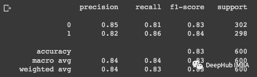
可以看到，标签 [0] 的精度更高，标签 [1] 的 f1 分数更高。在二分类的混淆矩阵中，我们看到了标签 [1] 的错误分类数据较少。

对于多标签分类

# Printing the model scores:
print(classification_report(y_test, y_pred))

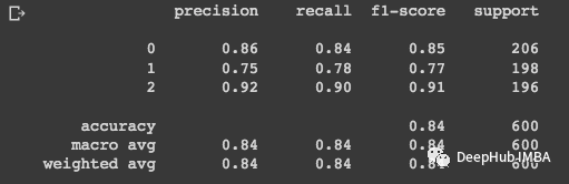
通过混淆矩阵，可以看到标签 [1] 是最难分类的，标签 [1] 的准确率、召回率和 f1 分数也是一样的。

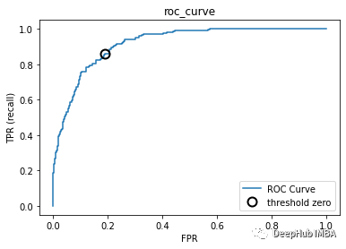
ROC和AUC

ROC 曲线，是一种图形表示，它说明了二元分类器系统在其判别阈值变化时的性能。ROC 曲线下的面积通常用于衡量测试的有用性，其中更大的面积意味着更有用的测试。ROC 曲线显示了假阳性率 (FPR) 与真阳性率 (TPR) 的对比。

#Get the values of FPR and TPR:
fpr, tpr, thresholds = roc_curve(y_test,logisticregression.decision_function(X_test))
plt.xlabel("FPR")
plt.ylabel("TPR (recall)")
plt.title("roc_curve");

# find threshold closest to zero:
close_zero = np.argmin(np.abs(thresholds))
plt.plot(fpr[close_zero], tpr[close_zero], 'o', markersize=10,
label="threshold zero", fillstyle="none", c='k', mew=2)
plt.legend(loc=4)

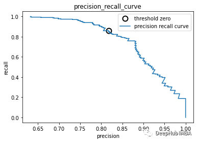
PR(precision recall )曲线

在P-R曲线中，Precision为横坐标，Recall为纵坐标。在ROC曲线中曲线越凸向左上角越好，在P-R曲线中，曲线越凸向右上角越好。P-R曲线判断模型的好坏要根据具体情况具体分析，有的项目要求召回率较高、有的项目要求精确率较高。P-R曲线的绘制跟ROC曲线的绘制是一样的，在不同的阈值下得到不同的Precision、Recall，得到一系列的点，将它们在P-R图中绘制出来，并依次连接起来就得到了P-R图。

PR 曲线只是一个图形，y 轴上有 Precision 值，x 轴上有 Recall 值。换句话说，PR 曲线在 y 轴上包含 TP/(TP+FN)，在 x 轴上包含 TP/(TP+FP)。

ROC 曲线是包含 x 轴上的 Recall = TPR = TP/(TP+FN) 和 y 轴上的 FPR = FP/(FP+TN) 的图。ROC曲线并且不会现实假阳性率与假阴性率，而是绘制真阳性率与假阳性率。

PR 曲线通常在涉及信息检索的问题中更为常见，不同场景对ROC和PRC偏好不一样，要根据实际情况区别对待。

#Get precision and recall thresholds:
precision, recall, thresholds = precision_recall_curve(y_test,logisticregression.decision_function(X_test))

# find threshold closest to zero:
close_zero = np.argmin(np.abs(thresholds))

#Plot curve:
plt.plot(precision[close_zero],     
         recall[close_zero], 
         'o', 
         markersize=10,
         label="threshold zero", 
         fillstyle="none", 
         c='k', 
         mew=2)
plt.plot(precision, recall, label="precision recall curve")
plt.xlabel("precision")
plt.ylabel("recall")
plt.title("precision_recall_curve");
plt.legend(loc="best")

作者：Carla Martins