
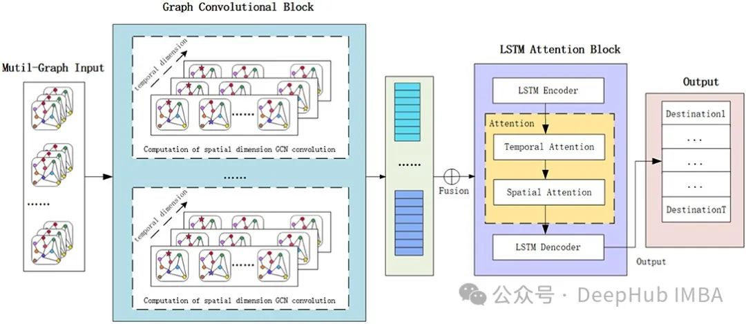
在我们周围的各个领域,从分子结构到社交网络,再到城市设计结构,到处都有相互关联的图数据。图神经网络(GNN)作为一种强大的方法,正在用于建模和学习这类数据的空间和图结构。它已经被应用于蛋白质结构和其他分子应用,例如药物发现,以及模拟系统,如社交网络。标准的GNN可以结合来自其他机器学习模型的想法,比如将GNN与序列模型结合——时空图神经网络(Spatail-Temporal Graph),能够捕捉数据的时间和空间依赖性。
对于时空图神经网络Spatail-Temporal Graph来说,最简单的描述就是在原来的Graph基础上增加了时间这一个维度,也就是说我们的Graph的节点特征是会随着时间而变化的。
GNN模型和序列模型(如简单RNN、LSTM或GRU)本身就复杂。结合这些模型以处理空间和时间依赖性是强大的,但也很复杂:难以理解,也难以实现。所以在这篇文章中,我们将深入探讨这些模型的原理,并实现一个相对简单的示例,以更深入地理解它们的能力和应用。
图神经网络(GNN)
我们先介绍一些入门的知识简要讨论GNN。
图G可以定义为G = (V, E),其中V是节点集,E是它们之间的边。
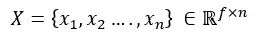
一个包含n个节点的图的特征矩阵,每个节点具有f个特征,是所有特征的连接:
GNN的关键问题是所有连接节点之间的消息传递,这种邻居特征转换和聚合可以写成:
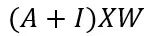
A是图的邻接矩阵,I是允许自连接的单位矩阵。虽然这不是完整的方程,但这已经可以说明可以学习不同节点之间空间依赖性的图卷积网络的基础。一个经典的图神经网络如下图所示:
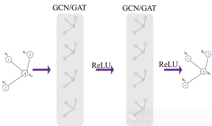
时空图神经网络 (ST-GNN)
ST-GNN中每个时间步都是一个图,并通过GCN/GAT网络传递,以获得嵌入数据空间相互依赖性的结果编码图。然后这些编码图可以像时间序列数据一样进行建模,只要保留每个时间步骤的数据的图结构的完整性。下图演示了这两个步骤,时间模型可以是从ARIMA或简单的循环神经网络或者是transformers的任何序列模型。
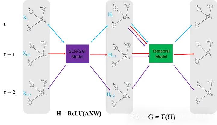
我们下面使用简单的循环神经网络来绘制ST-GNN的组件
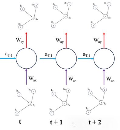
上面就是ST-GNN的基本原理,将GNN和序列模型(如RNN、LSTM、GRU、Transformers 等)结合。如果你已经熟悉这些序列和GNN模型,那么理论来说是非常简单的,但是实际操作的时候就会有一些复杂,所以我们下面将直接使用Pytorch实现一个简单的ST-GNN。
ST-GNN的Pytorch实现
首先要说明:为了用于演示我将使用大型科技公司的股市数据。虽然这些数据本质上不是图数据,但这种网络可能会捕捉到这些公司之间的相互依赖性,例如一个公司的表现(好或坏)可能反过来影响市场中其他公司的价值。但这只是一个演示,我们并不建议在股市预测中使用ST-GNN。
加载数据,直接使用yfinance里面什么都有
 importyfinanceasyf
 importdatetimeasdt
 importpandasaspd
 fromsklearn.preprocessingimportStandardScaler

 importplotly.graph_objsasgo
 fromplotly.offlineimportiplot
 importmatplotlib.pyplotasplt

 ############ Dataset download #################
 start_date=dt.datetime(2013,1,1)
 end_date=dt.datetime(2024,3,7)
 #loading from yahoo finance
 google=yf.download("GOOGL",start_date, end_date)
 apple=yf.download("AAPL",start_date, end_date)
 Microsoft=yf.download("MSFT", start_date, end_date)
 Amazon=yf.download("AMZN", start_date, end_date)
 meta=yf.download("META", start_date, end_date)
 Nvidia=yf.download("NVDA", start_date, end_date)
 data=pd.DataFrame({'google': google['Open'],'microsoft': Microsoft['Open'],'amazon': Amazon['Open'],
                      'Nvidia': Nvidia['Open'],'meta': meta['Open'], 'apple': apple['Open']})
 ############## Scaling data ######################
 scaler=StandardScaler()
 data_scaled=pd.DataFrame(scaler.fit_transform(data), columns=data.columns)
为了适应ST-GNN,所以我们要将数据进行转换以适应模型的要求
将标量时间序列数据集转换为图形数据结构是一个将传统数据转换为图神经网络可以处理的形式的关键步骤。这里描述的功能和类如下:
- 邻接矩阵的定义:
AdjacencyMatrix函数定义了图的邻接矩阵(连通性),这通常是基于手头物理系统的结构来完成的。然而,在这里,作者仅使用了一个全1矩阵,即所有节点都与所有其他节点相连。 - 股市数据集类:
StockMarketDataset类旨在为训练时空图神经网络(ST-GNNs)创建数据集。这个类中包含的方法有:- 数据序列生成:DatasetCreate方法生成数据序列。- 构造图边:_create_edges方法使用邻接矩阵构造图的边。- 生成数据序列:_create_sequences方法通过在输入的股市数据上滑动窗口来生成数据序列。
这种数据准备代码可以很容易地适应其他问题。这包括定义每个时间步的节点间的连接方式,并利用滑动窗口方法提取可以供模型学习的序列特征。通过这种方法,原本简单的时间序列数据被转化为具有复杂关系和时间依赖性的图形数据结构,从而可以使用图神经网络来进行更深入的分析和预测。
 defAdjacencyMatrix(L):
     AdjM=np.ones((L,L))
     returnAdjM

 classStockMarketDataset:
     def__init__(self, W,N_hist, N_pred):
         self.W=W
         self.N_hist=N_hist
         self.N_pred=N_pred
     defDatasetCreate(self):
         num_days, self.n_node=data_scaled.shape
         n_window=self.N_hist+self.N_pred
         edge_index, edge_attr=self._create_edges(self.n_node)
         sequences=self._create_sequences(data_scaled, self.n_node, n_window, edge_index, edge_attr)
         returnsequences
     def_create_edges(self, n_node):
         edge_index=torch.zeros((2, n_node**2), dtype=torch.long)
         edge_attr=torch.zeros((n_node**2, 1))
         num_edges=0
         foriinrange(n_node):
             forjinrange(n_node):
                 ifself.W[i, j] !=0:
                     edge_index[:, num_edges] =torch.tensor([i, j], dtype=torch.long)
                     edge_attr[num_edges, 0] =self.W[i, j]
                     num_edges+=1
         edge_index=edge_index[:, :num_edges]
         edge_attr=edge_attr[:num_edges]
         returnedge_index, edge_attr
     def_create_sequences(self, data, n_node, n_window, edge_index, edge_attr):
         sequences= []
         num_days, _=data.shape
         foriinrange(num_days):
             sta=i
             end=i+n_window
             full_window=np.swapaxes(data[sta:end, :], 0, 1)
             g=Data(x=torch.FloatTensor(full_window[:, :self.N_hist]),
                         y=torch.FloatTensor(full_window[:, self.N_hist:]),
                         edge_index=edge_index,
                         num_nodes=n_node)
             sequences.append(g)
         returnsequences
训练-验证-测试分割。
 fromtorch_geometric.loaderimportDataLoader

 deftrain_val_test_splits(sequences, splits):
     total=len(sequences)
     split_train, split_val, split_test=splits

     # Calculate split indices
     idx_train=int(total*split_train)
     idx_val=int(total* (split_train+split_val))
     indices= [iforiinrange(len(sequences)-100)]
     random.shuffle(indices)
     train= [sequences[index] forindexinindices[:idx_train]]
     val= [sequences[index] forindexinindices[idx_train:idx_val]]
     test= [sequences[index] forindexinindices[idx_val:]]
     returntrain, val, test
 '''Setting up the hyper paramaters'''
 n_nodes=6
 n_hist=50
 n_pred=10
 batch_size=32
 # Adjacency matrix
 W=AdjacencyMatrix(n_nodes)
 # transorm data into graphical time series
 dataset=StockMarketDataset(W, n_hist, n_pred)
 sequences=dataset.DatasetCreate()
 # train, validation, test split
 splits= (0.9, 0.05, 0.05)
 train, val, test=train_val_test_splits(sequences, splits)
 train_dataloader=DataLoader(train, batch_size=batch_size, shuffle=True, drop_last=True)
 val_dataloader=DataLoader(val, batch_size=batch_size, shuffle=True, drop_last=True)
 test_dataloader=DataLoader(test, batch_size=batch_size, shuffle=True, drop_last=True)
我们的模型包括一个GATConv和2个GRU层作为编码器,1个GRU层+全连接层作为解码器。GATconv是GNN部分,可以捕获空间依赖性,GRU层可以捕获数据的时间动态。代码包括大量的数据重塑,这样可以保证每一层的输入维度相同。这也是我们所说的ST-GNN实现中最复杂的部分,所以如果向具体了解输各层输入的维度,可以在向前传递的不同阶段打印x的形状,并将其与GRU和Linear层的预期输入尺寸的文档进行比较。
 importtorch
 importtorch.nn.functionalasF
 fromtorch_geometric.nnimportGATConv

 classST_GNN_Model(torch.nn.Module):
     def__init__(self, in_channels, out_channels, n_nodes,gru_hs_l1, gru_hs_l2, heads=1, dropout=0.01):
         super(ST_GAT, self).__init__()
         self.n_pred=out_channels
         self.heads=heads
         self.dropout=dropout
         self.n_nodes=n_nodes
         self.gru_hidden_size_l1=gru_hs_l1
         self.gru_hidden_size_l2=gru_hs_l2
         self.decoder_hidden_size=self.gru_hidden_size_l2
         # enconder GRU layers
         self.gat=GATConv(in_channels=in_channels, out_channels=in_channels,
                            heads=heads, dropout=dropout, concat=False)
         self.encoder_gru_l1=torch.nn.GRU(input_size=self.n_nodes,
                                         hidden_size=self.gru_hidden_size_l1, num_layers=1,
                                         bias=True)
         self.encoder_gru_l2=torch.nn.GRU(input_size=self.gru_hidden_size_l1,
                                            hidden_size=self.gru_hidden_size_l2, num_layers=1,
                                            bias=True)
         self.GRU_decoder=torch.nn.GRU(input_size=self.gru_hidden_size_l2, hidden_size=self.decoder_hidden_size,
                                         num_layers=1, bias=True, dropout=self.dropout)

         self.prediction_layer=torch.nn.Linear(self.decoder_hidden_size, self.n_nodes*self.n_pred, bias=True)

     defforward(self, data, device):
         x, edge_index=data.x, data.edge_index
         ifdevice=='cpu':
             x=torch.FloatTensor(x)
         else:
             x=torch.cuda.FloatTensor(x)
         x=self.gat(x, edge_index)
         x=F.dropout(x, self.dropout, training=self.training)
         batch_size=data.num_graphs
         n_node=int(data.num_nodes/batch_size)
         x=torch.reshape(x, (batch_size, n_node, data.num_features))
         x=torch.movedim(x, 2, 0)
         encoderl1_outputs, _=self.encoder_gru_l1(x)
         x=F.relu(encoderl1_outputs)
         encoderl2_outputs, h2=self.encoder_gru_l2(x)
         x=F.relu(encoderl2_outputs)
         x, _=self.GRU_decoder(x,h2)
         x=torch.squeeze(x[-1,:,:])
         x=self.prediction_layer(x)
         x=torch.reshape(x, (batch_size, self.n_nodes, self.n_pred))
         x=torch.reshape(x, (batch_size*self.n_nodes, self.n_pred))
         returnx
训练过程与pytorch中的任何网络训练过程几乎相同。
 importtorch
 importtorch.optimasoptim


 # Hyperparameters
 gru_hs_l1=16
 gru_hs_l2=16
 learning_rate=1e-3
 Epochs=50
 device='cuda'iftorch.cuda.is_available() else'cpu'
 model=ST_GNN_Model(in_channels=n_hist, out_channels=n_pred, n_nodes=n_nodes, gru_hs_l1=gru_hs_l1, gru_hs_l2=gru_hs_l2)
 pretrained=False
 model_path="ST_GNN_Model.pth"
 ifpretrained:
     model.load_state_dict(torch.load(model_path))
 optimizer=optim.Adam(model.parameters(), lr=learning_rate, weight_decay=1e-7)
 criterion=torch.nn.MSELoss()
 model.to(device)
 forepochinrange(Epochs):
     model.train()
     for_, batchinenumerate(tqdm(train_dataloader, desc=f"Epoch {epoch}")):
         batch=batch.to(device)
         optimizer.zero_grad()
         y_pred=torch.squeeze(model(batch, device))
         loss=criterion(y_pred.float(), torch.squeeze(batch.y).float())
         loss.backward()
         optimizer.step()
     print(f"Loss: {loss:.7f}")
模型训练完成了,下面就可视化模型的预测能力。对于每个数据输入,下面的代码预测模型输出,并随后绘制模型输出与基础真值的关系。
@torch.no_grad()
defExtract_results(model, device, dataloader, type=''):
model.eval()
model.to(device)
n=0
# Evaluate model on all data
fori, batchinenumerate(dataloader):
batch=batch.to(device)
ifbatch.x.shape[0] ==1:
pass
else:
withtorch.no_grad():
pred=model(batch, device)
truth=batch.y.view(pred.shape)
ifi==0:
y_pred=torch.zeros(len(dataloader), pred.shape[0], pred.shape[1])
y_truth=torch.zeros(len(dataloader), pred.shape[0], pred.shape[1])
y_pred[i, :pred.shape[0], :] =pred
y_truth[i, :pred.shape[0], :] =truth
n+=1
y_pred_flat=torch.reshape(y_pred, (len(dataloader),batch_size,n_nodes,n_pred))
y_truth_flat=torch.reshape(y_truth,(len(dataloader),batch_size,n_nodes,n_pred))
returny_pred_flat, y_truth_flat
defplot_results(predictions,actual, step, node):
predictions=torch.tensor(predictions[:,:,node,step]).squeeze()
actual=torch.tensor(actual[:,:,node,step]).squeeze()
pred_values_float=torch.reshape(predictions,(-1,))
actual_values_float=torch.reshape(actual, (-1,))
scatter_trace=go.Scatter(
x=actual_values_float,
y=pred_values_float,
mode='markers',
marker=dict(
size=10,
opacity=0.5,
color='rgba(255,255,255,0)',
line=dict(
width=2,
color='rgba(152, 0, 0, .8)',
)
),
name='Actual vs Predicted'
)
line_trace=go.Scatter(
x=[min(actual_values_float), max(actual_values_float)],
y=[min(actual_values_float), max(actual_values_float)],
mode='lines',
marker=dict(color='blue'),
name='Perfect Prediction'
)
data= [scatter_trace, line_trace]
layout=dict(
title='Actual vs Predicted Values',
xaxis=dict(title='Actual Values'),
yaxis=dict(title='Predicted Values'),
autosize=False,
width=800,
height=600
)
fig=dict(data=data, layout=layout)
iplot(fig)
y_pred, y_truth=Extract_results(model, device, test_dataloader, 'Test')
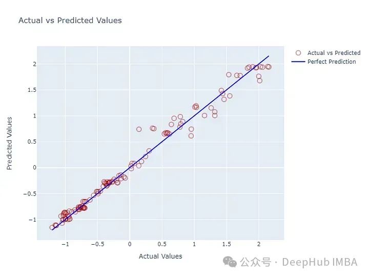
plot_results(y_pred, y_truth,9,0) # timestep, node
对于6个节点(公司),给出过去50个值,做出10个预测。下面是第一个节点的第10步预测与真值的图。看起来看不错,但并不一定意味着就很好。因为对于时间序列数据,下一个值的最佳估计量总是前一个值。如果没有得到很好的训练,这些模型可以输出与输入数据的最后一个值相似的值,而不是捕获时间动态。
对于给定的节点,我们可以绘制历史输入、预测和真值进行比较,查看预测是否捕获了模式。
 @torch.no_grad()
 defforecastModel(model, device, dataloader, node):
     model.eval()
     model.to(device)
     fori, batchinenumerate(dataloader):
         batch=batch.to(device)
         withtorch.no_grad():
             pred=model(batch, device)
         truth=batch.y.view(pred.shape)
         # the shape should [batch_size, nodes, number of predictions]
         truth=torch.reshape(truth, [batch_size, n_nodes,n_pred])
         pred=torch.reshape(pred, [batch_size, n_nodes,n_pred])
         x=batch.x
         x=torch.reshape(x, [batch_size, n_nodes,n_hist])

         y_pred=torch.squeeze(pred[0, node, :])
         y_truth=torch.squeeze(truth[0,node,:])
         y_past=torch.squeeze(x[0, node, :])
         t_range= [tfortinrange(len(y_past))]
         break
     t_shifted= [t_range[-1]+1+tfortinrange(len(y_pred))]
     trace1=go.Scatter(x=t_range, y=y_past, mode="markers", name="Historical data")
     trace2=go.Scatter(x=t_shifted, y=y_pred, mode="markers", name="pred")
     trace3=go.Scatter(x=t_shifted, y=y_truth, mode="markers", name="truth")
     layout=go.Layout(title="forecasting", xaxis=dict(title='time'),
                        yaxis=dict(title='y-value'), width=1000, height=600)

     figure=go.Figure(data= [trace1, trace2, trace3], layout=layout)
     iplot(figure)
 forecastModel(model, device, test_dataloader, 0)
![]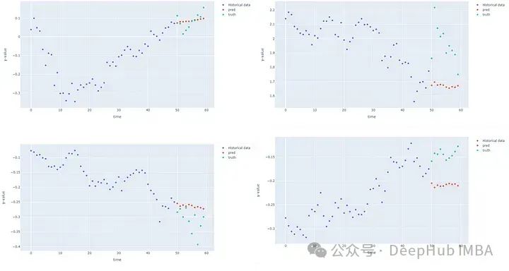
第一个节点(Google)在测试数据集的4个不同点上的预测实际上比我想象的要好,其他的看来不怎么样。
总结
我的理解是未来的股票价格不能通过单纯的历史价值自回归来预测,因为股票是由现实世界的事件决定的,这并没有体现在历史价值中。这也就是我们在前面说的不建议在股市预测中使用ST-GNN,我们使用这个数据集只是因为它容易获取。最后不要忘集我们本篇文章的目的,学习ST-GNN的基本概念,以及通过Pytorch代码实现来了解ST-GNN的工作原理。
作者:Najib Sharifi