
线性方程组的求解包括直接法和迭代法,其中迭代法包括传统的高斯消元法,最速下降法,牛顿法,雅克比迭代法,共轭梯度法,以及智能启发式算法求解法和神经网络学习算法,传统算法可以相互组合改进,智能仿生启发式算法包括粒子群算法,遗传算法,模拟退火算法,布谷鸟算法狼群算法,樽海鞘算法,天牛须算法等各种启发算法都可以求解,神经网络算法包括BP神经网络,RBF神经网络,DBN神经网络,CNN神经网络等机器学习算法,总之求解方法凡凡总总,本文仅介绍10种方法如下:
** 一、直接法**
直接法就是经过有限步算术运算,可求得线性方程组精确解的方法(若计算过程中没有舍入误差)。常用于求解低阶稠密矩阵方程组及某些大型稀疏矩阵方程组(如大型带状方程组)。MATLAB代码如下:
** clc
clear
close all
q = [2 0 2 7
7 7 1 3
3 8 2 0
2 7 7 7];
b = [1;3;3;8];
x = q\b**
** 求解结果 **x =
** 0.9505
-0.5099
2.1139
-0.7327**
** 二、高斯消元法**
数学上,高斯消元法(或译:高斯消去法),是线性代数规划中的一个算法,可用来为线性方程组求解,MATALB代码如下:
clc
clear
close all
q = [2 0 2 7
7 7 1 3
3 8 2 0
2 7 7 7];
b = [1;3;3;8];
n=length(q);
a=[q,b];
for k=1:n-1
maxa=max(abs(a(k:n,k)));
if maxa==0
return;
end
** for i=k:n**
** if abs(a(i,k))==maxa**
** y=a(i,k:n+1);a(i,k:n+1)=a(k,k:n+1);a(k,k:n+1)=y;**
** break;
end
end**
** for i=k+1:n**
** l(i,k)=a(i,k)/a(k,k);**
** a(i,k+1:n+1)=a(i,k+1:n+1)-l(i,k).a(k,k+1:n+1);*
** end
end**
if a(n,n)==0
return
end
*x(n)=a(n,n+1)/a(n,n);
for i=n-1:-1:1
x(i)=(a(i,n+1)-sum(a(i,i+1:n).x(i+1:n)))/a(i,i);
**end
fprintf('x= %10.9f\n', x) **
**求解结果 x = 0.9505 **
** -0.5099 **
** 2.1139 **
** -0.7327**
** 三、共轭梯度法**
** clc*共轭梯度法(Conjugate Gradient)是介于最速下降法与牛顿法之间的一个方法,它仅需利用一阶导数信息,但克服了最速下降法收敛慢的缺点,又避免了牛顿法需要存储和计算Hesse矩阵并求逆的缺点,MATLAB代码如下
*clear
close all
DIM=4;
tic
A=10rand(DIM);% A元素是0-100
for i=1:DIM
A(i,i)=sum(abs(A(i,:)))+25*rand(1); %对角占优的量为0~25
end
b=zeros(DIM,1);
for i=1:DIM;
x=0;
for r=1:DIM;
x=x+A(i,r);
end
b(i,1)=x;
end %产生b矩阵,b中的元素为A中对应行的和,目的是使方程解全为 1*
jd=10^-6;
x0=zeros(DIM,1); %初始迭代矩阵
r=b-Ax0;%剩余向量
p=r;
ak=dot(r,r)/dot(p,Ap);
y=x0+akp; %迭代公式
r1=r-akAp;
bk=dot(r1,r1)/dot(r,r);
p1=r1+bkp;
s=1; %迭代次数
while norm(y-x0)>=jd&&s<3000; %迭代条件
x0=y;
p=p1;
r=r1;
ak=dot(r,r)/dot(p,Ap);
y=x0+akp; %迭代公式
r1=r-akAp;
bk=dot(r1,r1)/dot(r,r);
p1=r1+bk*p;
s=s+1;
end
t=1:DIM;
aerr=abs(y'-1)/1;
plot(t,aerr);
title('绝对误差图')
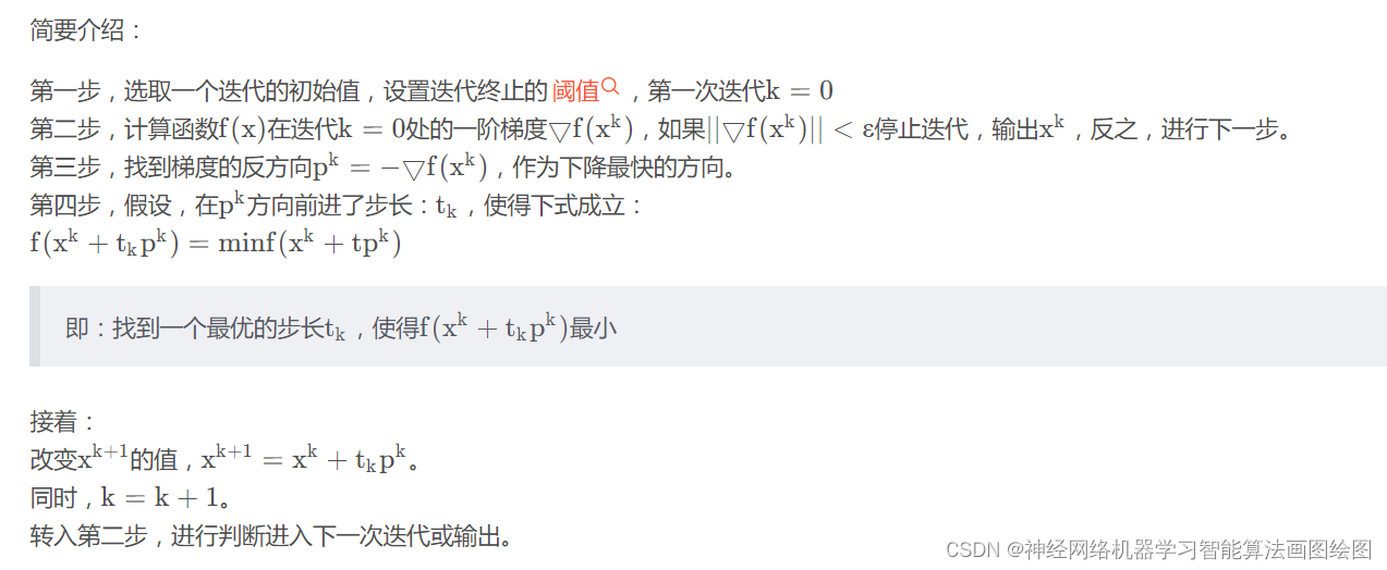
四、最速下降法
简要介绍:
 MATLAB代码如下:
n = 0;
x0 = [0 0 0 0]';
DIM=4;
tic
A=10rand(DIM);% A元素是0-100
for i=1:DIM
A(i,i)=sum(abs(A(i,:)))+25rand(1); %对角占优的量为0~25
end
b=zeros(DIM,1);
for i=1:DIM;
x=0;
for r=1:DIM;
x=x+A(i,r);
end
b(i,1)=x;
end %产生b矩阵,b中的元素为A中对应行的和,目的是使方程解全为 1
r = A*x0 - b;
p = -r;
eps=10^-3;
t = cputime;
**while (norm(r,2) > eps)&&n<2000
  alpha = (r'*r)/(p'*A*p);
     x0 = x0 + alpha*p   ;
     r1 =  r + alpha*A*p ;
   beta = (r1'*r1)/(r'*r);
      p = -r1 + beta*p   ;
      r = r1;
      n = n+1;
end
time = cputime - t;**
五、雅克比迭代法
考虑线性方程组**A*****x = *****b**时,一般当**A**为低阶稠密矩阵时,用主元消去法解此方程组是有效方法。但是,对于由工程技术中产生的大型稀疏矩阵方程组(**A**的阶数很高,但零元素较多,例如求某些偏微分方程数值解所产生的线性方程组),利用迭代法求解此方程组就是合适的,在计算机内存和运算两方面,迭代法通常都可利用A中有大量零元素的特点。雅克比迭代法就是众多迭代法中比较早且较简单的一种,其命名也是为纪念普鲁士著名数学家雅可比。MATLAB代码如下:
A = [2 0 2 7
7 7 1 3
3 8 2 0
2 7 7 7];
b = [1;3;3;8];
x0=[0 0 0 0]';
eps= 1.0e-6;
 M  = 1000;
D=diag(diag(A)); %求A的对角矩阵
L=-tril(A,-1); %求A的下三角阵
U=-triu(A,1); %求A的上三角阵
B=D(L+U);
f=D\b;
x=Bx0+f;
n=0; %迭代次数
while norm(x-x0)>=eps
x0=x;
x=Bx0+f;
n=n+1;
if(n>=M)
disp('Warning: 迭代次数太多,可能不收敛!');
return;
end
x
end
六、超松弛迭代法
一般而言,因雅可比迭代收敛速度不够快,所以在工程中应用不多。并且在雅可比迭代收敛速
度很慢的情况下,通常高斯-赛德尔方法也不会很快。我们可以对高斯-赛德尔方法做出一定的
修改,来提高收敛速度。我们介绍超松弛迭代法可以提高收敛速度,MATLAB代码如下
clc
clear
close all
DIM=4;
A=10rand(DIM);% A元素是0-100
for i=1:DIM
A(i,i)=sum(abs(A(i,:)))+25rand(1); %对角占优的量为0~25
end
b=zeros(DIM,1);
x0=[10 10 10 10]';
w=1.025;
tol = 10^-10;
D=diag(diag(A));
L = -tril(A,-1);
U = -triu(A,1);
B = (D - w * L) \ ((1 - w) * D + w * U);
g = (D - w * L) \ b * w;
x = B * x0 +g;
n=1;
while norm(x - x0) >= tol
x0 = x;
x= B * x0 + g;
n = n + 1;
end
七、粒子群算法
直接发和迭代法,都有一定的适用范围,对应复杂的方程组,往往没法收敛,启发式算法,比如粒子群,可以自适应的对方程组的解进行求解,对复杂的方程组的求解精度一般更高,代码通用性更强,PSO是由Kennedy和Eberhart共同提出,最初用于模拟社会行为,作为鸟群或鱼群中有机体运动的形式化表示。自然界中各种生物体均具有一定的群体行为,Kennedy和Eberhart的主要研究方向之一是探索自然界生物的群体行为,从而在计算机上构建其群体模型。PSO是一种元启发式算法,因为它很少或没有对被优化的问题作出假设,并且能够对非常大候选解决方案空间进行搜索,算法的主要参数包括,最大迭代次数,种群个数,学习因子,权重因子,种群位置,种群速度,个体最优解,全局最优解,MATLAB代码如下
clc
clear
close all
format long
warning off
set(0,'defaultfigurecolor','w')
xmax = [100 6 ];
xmin = [60 2 ];
vmax = 0.1*xmax;
vmin = -vmax;
m=2;
%程序初始化
% global popsize; %种群规模
gen=10; %设置进化代数
popsize=300; %设置种群规模大小
best_in_history(gen)=inf; %初始化全局历史最优解
best_in_history(:)=inf; %初始化全局历史最优解
best_fitness=inf;
fz = zeros(gen,5);
%设置种群数量
pop1 = zeros(popsize,m);
pop2 = zeros(popsize,m);
pop3 = zeros(popsize,m);
pop6 = zeros(gen,m);%存储解码后的每代最优粒子
pop7 = zeros(popsize,m);%存储更新解码后的粒子的位置
pop8=zeros(popsize,5);%保存
for ii1=1:popsize
pop1(ii1,:)=funx(xmin,xmax,m); %初始化种群中的粒子位置,
pop3(ii1,:)=pop1(ii1,:); %初始状态下个体最优值等于初始位置
pop2(ii1,:)=funv(vmax,m); %初始化种群微粒速度,
pop4(ii1,1)=inf;
pop5(ii1,1)=inf;
end
pop0=pop1;
c1=2;
c2=2;
gbest_x=pop1(end,:);
% pop1(1:size(num,1),:) = num; %全局最优初始值为种群第一个粒子的位置
for exetime=1:gen
 ww = 0.7*(gen-exetime)/gen+0.2;
 for ii4=1:popsize

     pop2(ii4,:)=(ww*pop2(ii4,:)+c1*rand(1,m).*(pop3(ii4,:)-pop1(ii4,:))+c2*rand(1,m).*(gbest_x-pop1(ii4,:)));    %更新速度
     for jj = 1:m
         if  pop2(ii4,jj)<vmin(jj)
             pop2(ii4,jj)=vmin(jj);
         elseif pop2(ii4,jj)>vmax(jj)
             pop2(ii4,jj)=vmax(jj);
         end
     end
 end
 %更新粒子位置
 for ii5=1:popsize
     pop1(ii5,:)=pop1(ii5,:)+pop2(ii5,:);
     for jj2 = 1:m
         if  pop1(ii5,jj2)>xmax(jj2)
             pop1(ii5,jj2) = xmax(jj2);
         elseif pop1(ii5,jj2)<xmin(jj2)
             pop1(ii5,jj2)=xmin(jj2);
         end
     end
% if rand>0.85
% k=ceil(m*rand);
% pop1(ii5,k) = (xmax( k)-xmin(k)).*rand(1,1)+xmin(k);
% end
% if pop5(ii5)>sum(pop5)/popsize
% pop1(ii5,:) = (xmax(1,m)-xmin(1,m)).*rand(1,m)+xmin(1,m);
% end
end
for jj2 = 1:m
if pop1(ii5,jj2)>xmax(jj2)
pop1(ii5,jj2) = xmax(jj2);
elseif pop1(ii5,jj2)<xmin(jj2)
pop1(ii5,jj2)=xmin(jj2);
end
end
if exetime-1>0
plot(1:length(best_in_history(1:exetime-1)),best_in_history(1:exetime-1),'b-','LineWidth',1.5);
xlabel('迭代次数')
ylabel('适应度')
title('粒子群算法')
hold on;
pause(0.1)
end
 pop1(end,:) = gbest_x;
 %计算适应值并赋值
 for ii3=1:popsize
     [my,mx,ff] = fun2(pop1(ii3,:));
     %          [my,mx] = fun2(gbest_x,num,xmax,xmin);
     pop5(ii3,1)=my;
     pop7(ii3,:) = mx;
     pop8(ii3,:) = ff;
     if  pop4(ii3,1)>pop5(ii3,1)    %若当前适应值优于个体最优值,则进行个体最优信息的更新
         pop4(ii3,1)=pop5(ii3,1);          %适值更新
         pop3(ii3,:)=pop1(ii3,:);      %位置坐标更新
     end
 end

 %计算完适应值后寻找当前全局最优位置并记录其坐标
 if  best_fitness>min(pop4(:,1))
     best_fitness=min(pop4(:,1))  ;  %全局最优值
     ag = [];
     ag =find(pop4(:,1)==min(pop4(:,1)));

     gbest_x(1,:)=(pop1(ag(1),:));    %全局最优粒子的位置
     fz(exetime,:) = pop8(ag(1),:);
     pop6(exetime,:) = pop7(ag(1),:);
 else
     fz(exetime,:) = fz(exetime-1,:);
     if exetime>1
         pop6(exetime,:) = pop6(exetime-1,:);
     end
 end
 best_in_history(exetime)=best_fitness;  %记录当前全局最优
end
figure
plot(pop0(:,1),pop0(:,2),'k*')
xlabel('X')
ylabel('Y')
title('初始种群')
set(gca,'fontsize',12)
% load maydata.mat
figure
plot(pop1(:,1),pop1(:,2),'k*')
xlabel('X')
ylabel('Y')
title('收敛后的种群')
set(gca,'fontsize',12)
[X,Y] = meshgrid(60:100,2:0.05:6);
Z = -29310 + 1621X -473.5Y -31.7X.^2 + 21.63X.Y + 0.2722X.^3 -0.3143X.^2.Y -0.0008683X.^4 + 0.001494X.^3.*Y;
x1 = pop0(:,1);
y1 = pop0(:,2);
f21 = -29310 + 1621x1 -473.5y1 -31.7x1.^2 + 21.63x1.y1 + 0.2722x1.^3 -0.3143x1.^2.y1 -0.0008683x1.^4 +0.001494x1.^3.*y1;
x2 = pop1(:,1);
y2 = pop1(:,2);
f22 = -29310 + 1621x2 -473.5y2 -31.7x2.^2 + 21.63x2.y2 + 0.2722x2.^3 -0.3143x2.^2.y2 -0.0008683x2.^4 +0.001494x2.^3.*y2;
[X,Y] = meshgrid(60:100,2:0.05:6);
Z2 = 190 - 12.1X - 16.61Y + 0.3042X.^2 + 0.8998X.Y -0.003729X.^3 -0.01836X.^2.Y +0.00002218X.^4 + 0.0001653X.^3.Y - 0.0000000509X.^5 - 0.0000005522X.^4.Y;
x1 = pop0(:,1);
y1 = pop0(:,2);
f23 = 190 - 12.1x1 - 16.61y1 + 0.3042x1.^2 + 0.8998x1.y1 -0.003729x1.^3 -0.01836x1.^2.y1 +0.00002218x1.^4 + 0.0001653x1.^3.y1 - 0.0000000509x1.^5 - 0.0000005522x1.^4.y1;
x2 = pop1(:,1);
y2 = pop1(:,2);
f24 = 190 - 12.1x2 - 16.61y2 + 0.3042x2.^2 + 0.8998x2.y2 -0.003729x2.^3 -0.01836x2.^2.y2 +0.00002218x2.^4 + 0.0001653x2.^3.y2 - 0.0000000509x2.^5 - 0.0000005522*x2.^4.*y2;
[X,Y] = meshgrid(60:100,2:0.05:6);
Z3 = 3.327 + 0.2373X -0.5549Y -0.01062X.^2 + 0.02165X.Y + 0.0001393X.^3 -0.0003284X.^2.Y -0.0000005832X.^4 + 0.000001639X.^3.Y;
x1 = pop0(:,1);
y1 = pop0(:,2);
f25 = 3.327 + 0.2373x1 -0.5549y1 -0.01062x1.^2 + 0.02165x1.y1 + 0.0001393x1.^3 -0.0003284x1.^2.y1 -0.0000005832x1.^4 + 0.000001639x1.^3.y1;
x2 = pop1(:,1);
y2 = pop1(:,2);
f26 = 3.327 + 0.2373x2 -0.5549y2 -0.01062x2.^2 + 0.02165x2.y2 + 0.0001393x2.^3 -0.0003284x2.^2.y2 -0.0000005832x2.^4 + 0.000001639x2.^3.*y2;
[X,Y] = meshgrid(60:100,2:0.05:6);
Z4 = 22680 -1634X -3160Y + 46.03X.^2 +159.3X.Y -0.6327X.^3 -2.965X.^2.Y +0.004249X.^4 +0.02432X.^3.Y -0.00001116X.^5 - 0.00007448X.^4.Y;
x1 = pop0(:,1);
y1 = pop0(:,2);
f27 = 22680 -1634x1 -3160y1 + 46.03x1.^2 +159.3x1.y1 -0.6327x1.^3 -2.965x1.^2.y1 +0.004249x1.^4 +0.02432x1.^3.y1 -0.00001116x1.^5 - 0.00007448x1.^4.y1;
x2 = pop1(:,1);
y2 = pop1(:,2);
f28 = 22680-1634x2 -3160y2 + 46.03x2.^2 +159.3x2.y2 -0.6327x2.^3 -2.965x2.^2.y2 +0.004249x2.^4 +0.02432x2.^3.y2 -0.00001116x2.^5 - 0.00007448x2.^4.y2;
[X,Y] = meshgrid(60:100,2:0.05:6);
Z5 = -46.14 +2.441X + 0.2536Y -0.04762X.^2 -0.007813X.Y + 0.0004074X.^3 + 0.00009046X.^2.Y -0.000001289X.^4 -0.0000003687X.^3.Y;
x1 = pop0(:,1);
y1 = pop0(:,2);
f29 = -46.14 +2.441x1 + 0.2536y1 -0.04762x1.^2 -0.007813x1.y1 + 0.0004074x1.^3 + 0.00009046x1.^2.y1 -0.000001289x1.^4 -0.0000003687x1.^3.y1;
x2 = pop1(:,1);
y2 = pop1(:,2);
f30 = -46.14 +2.441x2 + 0.2536y2 -0.04762x2.^2 -0.007813x2.y2 + 0.0004074x2.^3 + 0.00009046x2.^2.y2 -0.000001289x2.^4 -0.0000003687x2.^3.*y2;
figure
surf(X,Y,Z)
hold on
shading interp
plot3(x1,y1,f21,'ro','MarkerFaceColor','r')
xlabel('转速n(r/min)')
ylabel('牵引速度v_q(m/min)')
zlabel('切削面积_5(cm^2)')
title('初始种群')
set(gca,'fontsize',12)
figure
surf(X,Y,Z)
shading interp
hold on
plot3(x2,y2,f22,'ro','MarkerFaceColor','r')
xlabel('转速n(r/min)')
ylabel('牵引速度v_q(m/min)')
zlabel('应力峰值S_5(Mpa)')
title('收敛后的种群')
set(gca,'fontsize',12)
figure
surf(X,Y,Z2)
hold on
shading interp
plot3(x1,y1,f23,'ro','MarkerFaceColor','r')
xlabel('转速n(r/min)')
ylabel('牵引速度v_q(m/min)')
zlabel('载荷波动系数\delta_5')
title('初始种群')
set(gca,'fontsize',12)
figure
surf(X,Y,Z2)
shading interp
hold on
plot3(x2,y2,f24,'ro','MarkerFaceColor','r')
xlabel('转速n(r/min)')
ylabel('牵引速度v_q(m/min)')
zlabel('载荷波动系数\delta_5')
title('收敛后的种群')
set(gca,'fontsize',12)
figure
surf(X,Y,Z3)
hold on
shading interp
plot3(x1,y1,f25,'ro','MarkerFaceColor','r')
xlabel('转速n(r/min)')
ylabel('牵引速度v_q(m/min)')
zlabel('截割比能耗H_w_5(kW·h/m^3)')
title('初始种群')
set(gca,'fontsize',12)
figure
surf(X,Y,Z3)
shading interp
hold on
plot3(x2,y2,f26,'ro','MarkerFaceColor','r')
xlabel('转速n(r/min)')
ylabel('牵引速度v_q(m/min)')
zlabel('截割比能耗H_w_5(kW·h/m^3)')
title('收敛后的种群')
set(gca,'fontsize',12)
figure
surf(X,Y,Z4)
hold on
shading interp
plot3(x1,y1,f27,'ro','MarkerFaceColor','r')
xlabel('转速n(r/min)')
ylabel('牵引速度v_q(m/min)')
zlabel('载荷峰值Q_s_5(kN/m)')
title('初始种群')
set(gca,'fontsize',12)
figure
surf(X,Y,Z4)
shading interp
hold on
plot3(x2,y2,f28,'ro','MarkerFaceColor','r')
xlabel('转速n(r/min)')
ylabel('牵引速度v_q(m/min)')
zlabel('滚筒负载Q_s_5(×10^4N/m)')
title('收敛后的种群')
set(gca,'fontsize',12)
figure
surf(X,Y,Z5)
hold on
shading interp
plot3(x1,y1,f29,'ro','MarkerFaceColor','r')
xlabel('转速n(r/min)')
ylabel('牵引速度v_q(m/min)')
zlabel('装煤率\eta_5(%)')
title('初始种群')
set(gca,'fontsize',12)
figure
surf(X,Y,Z5)
shading interp
hold on
plot3(x2,y2,f30,'ro','MarkerFaceColor','r')
xlabel('转速n(r/min)')
ylabel('牵引速度v_q(m/min)')
zlabel('装煤率\eta_5(%)')
title('收敛后的种群')
set(gca,'fontsize',12)
[f,mx,ff,ff1] = fun3(gbest_x);
figure
for ii = 1
plot(fz(:,ii),'k-o','LineWidth',1.5)
hold on
end
xlabel('迭代次数')
ylabel('装煤率\eta_5适应度')
set(gca,'fontsize',12)
xlim([1 9])
figure
for ii = 2
plot (fz(:,ii),'r-o','LineWidth',1.5)
hold on
end
xlabel('迭代次数')
ylabel('切削面积S_5适应度')
set(gca,'fontsize',12)
xlim([1 9])
figure
for ii = 3
plot(fz(:,ii),'b-o','LineWidth',1.5)
hold on
end
xlabel('迭代次数')
ylabel('载荷波动系数\delta_5适应度')
set(gca,'fontsize',12)
xlim([1 9])
figure
for ii = 4
plot(fz(:,ii),'g-o','LineWidth',1.5)
hold on
end
xlabel('迭代次数')
ylabel('滚筒负载Q_s_5适应度')
set(gca,'fontsize',12)
xlim([1 9])
figure
for ii = 5
plot(fz(:,ii),'m-o','LineWidth',1.5)
hold on
end
xlabel('迭代次数')
ylabel('截割比能耗H_w_5适应度')
set(gca,'fontsize',12)
xlim([1 9])
基于粒子群的复杂方程组求解-机器学习文档类资源-CSDN文库 https://download.csdn.net/download/abc991835105/86962101
八、遗传算法
遗传算法的基本运算过程如下:
(1)初始化:设置进化代数计数器t=0,设置最大进化代数T,随机生成M个个体作为初始群体P(0)。
(2)个体评价:计算群体P(t)中各个个体的适应度。
(3)选择运算:将选择算子作用于群体。选择的目的是把优化的个体直接遗传到下一代或通过配对交叉产生新的个体再遗传到下一代。选择操作是建立在群体中个体的适应度评估基础上的。
(4)交叉运算:将交叉算子作用于群体。遗传算法中起核心作用的就是交叉算子。
(5)变异运算:将变异算子作用于群体。即是对群体中的个体串的某些基因座上的基因值作变动。群体P(t)经过选择、交叉、变异运算之后得到下一代群体P(t+1)。
(6)终止条件判断:若t=T,则以进化过程中所得到的具有最大适应度个体作为最优解输出,终止计算。
遗传操作包括以下三个基本遗传算子(genetic operator):选择(selection);交叉(crossover);变异(mutation)。
matlab代码如下:
clc
clear
close all
Size=300; %种群规模
G=50; %最大迭代次数
CodeL=10; %染色体长度
dim = 4;
umax=[30 30 30 30]; %上限
umin=[-30 -30 -30 -30]; %下限
E=round(rand(Size,dim*CodeL)); %种群初始化
zbestf = 0;
bfi= zeros(G,1);
bfi(1) = 200;
%主循环
for k=1:1:G
time(k)=k;
[F,x1,x2,x3,x4] = fun(E,umax,umin,Size);
%**** Step 1 : Evaluate BestJ ******
fi=F; %适应度值
[Oderfi,Indexfi]=sort(fi); %排序
Bestfi=Oderfi(Size); %最大值
BestS=E(Indexfi(Size),:); %最优染色体
bfi(k)=Bestfi;
if zbestf<Bestfi
zbestf = Bestfi;
zbest = BestS;
end
%****** Step 2 : 选择******
fi_sum=sum(fi);
fi_Size=(Oderfi/fi_sum)*Size;
fi_S=floor(fi_Size);        %被选择概率

kk=1;
for ii=1:1:Size
   for jj=1:1:fi_S(ii)
       TempE(kk,:)=E(Indexfi(ii),:);
       kk=kk+1;
   end
end
%************ Step 3 : 交叉 ************
pc=0.60; %交叉概率
n=ceil(CodeL*rand);
for ii=1:2:(Size-1)
 for jj=n:1:dim*CodeL
     temp=rand;
     if pc>temp
        TempE(ii,jj)=E(ii+1,jj);
        TempE(ii+1,jj)=E(ii,jj);
     end
 end
end
TempE(Size,:)=BestS;
E=TempE;
%************ Step 4: 变异 ************** **
**pm=0.8; %变异概率
for ii=1:1:Size
mx = round((dim*CodeL-1)rand()+1);
my = randperm(dimCodeL);
temp=rand;
if pm>temp %
for jj = 1:mx
if TempE(ii,jj)==0
TempE(ii,jj)=1;
else
TempE(ii,jj)=0;
end
end
end
end
**
TempE(Size,:)=BestS;
E=TempE;
end
zbfi = bfi(1);
for ii = 2:size(bfi)
if zbfi(ii-1)<=bfi(ii)
zbfi = [zbfi bfi(ii)];
elseif zbfi(ii-1)>bfi(ii)
zbfi = [zbfi zbfi(ii-1)];
end
end
[F,xx1,xx2,x3,x4] = fun(zbest,umax,umin,1);
zbest
Mmin_Value=1./zbestf
gbest_x = [xx1 xx2 x3 x4]
figure(2);
plot(time,1./zbfi);
xlabel('迭代次数');
ylabel(' Rosenbrock');
title('遗传算法')
x1 = -30:30;
x2 = -30:30;
[x,y] = meshgrid(x1,x2);
f = zeros(61,61);
for ii = 1:61
for jj = 1:61
f(ii,jj) = sum((x(ii,jj)-y(ii,jj)).^2)+sum(([x(ii,jj) y(ii,jj)]-1).^2);
end
end
figure
surf(x,y,f)
shading interp
hold on
plot3(xx1,xx2,Mmin_Value,'ro')
hold off
xlabel('x')
ylabel('y')
zlabel('Rosenbrock')
title('遗传算法')
基于MATLAB的遗传算法求解方程组-机器学习文档类资源-CSDN文库 https://download.csdn.net/download/abc991835105/86966265
九、鲸鱼算法
鲸鱼算法是一种模仿鲸鱼捕食行为产生的算法,鲸鱼是一种群组哺乳海洋动物,常常通过群体合作对猎物进行围捕和捕猎,鲸鱼算法是一种比较新的算法,应用相对其他算法要稍很多,比灰狼算法还要晚些,MATALB代码如下:
*clc
clear
close all
load maydata.mat
xa = ax;
SearchAgents_no=3; % 变量维数
Function_name='goal_function'; % 适应度函数
Max_iteration=100; %最大迭代次数
lb = [-5 -5 95];
ub = [5 5 105];
dim = 3;
[Best_score,Best_pos,WOA_cg_curve]=WOA(SearchAgents_no,Max_iteration,lb,ub,dim,xa);
theta = 0:pi/100:10pi;
x1 = Best_pos(1)*theta.*cos(theta);
y1 = Best_pos(1)*theta.sin(theta);
z1 = Best_pos(2)theta+Best_pos(3);
figure
plot3(xa(:,1),xa(:,2),xa(:,3),'bo')
hold on
plot3(x1,y1,z1,'r-')
hold off
xlabel('x')
ylabel('y')
zlabel('z')
legend('实际散点','鲸鱼算法拟合曲线')
figure
semilogy(WOA_cg_curve,'Color','r')
title('WOA')
xlabel('迭代次数');
ylabel('目标函数值');
axis tight
grid on
box on
基于MATLAB的鲸鱼算法多目标优化,基于MATLAB的鲸鱼算法多方程组求解-机器学习文档类资源-CSDN文库 https://download.csdn.net/download/abc991835105/86966822
十、BP神经网络算法
BP神经网络算法是模仿人类神经元开发出来的算法,是较早更成熟的一种基础机器学习算法,算法结构简单,但是发展很完善,适用性和实用性很强,工具箱强大完善,可以处理解决很多问题,MATALB求解方程组的解代码如下;
clc
clear
close all
%% 训练数据预测数据提取及归一化
%找出训练数据和预测数据
input_train=[2 0 2 7
7 7 1 3
3 8 2 0
2 7 7 7]';
output_train=[-11 -18 -13 -23];
input_test=input_train;
output_test=output_train;
%选连样本输入输出数据归一化
[inputn,inputps]=mapminmax(input_train);
[outputn,outputps]=mapminmax(output_train);
%% 网络结构初始化
innum=4;
midnum=4;
outnum=1;
%权值初始化
w1=rands(midnum,innum);
b1=rands(midnum,1);
w2=rands(midnum,outnum);
b2=rands(outnum,1);
w2_1=w2;w2_2=w2_1;
w1_1=w1;w1_2=w1_1;
b1_1=b1;b1_2=b1_1;
b2_1=b2;b2_2=b2_1;
%学习率
xite=0.1;
alfa=0.01;
loopNumber=200;
I=zeros(1,midnum);
Iout=zeros(1,midnum);
FI=zeros(1,midnum);
dw1=zeros(innum,midnum);
db1=zeros(1,midnum);
**%% 网络训练
E=zeros(1,loopNumber);
for ii=1:loopNumber
E(ii)=0;
for i=1:1:4
%% 网络预测输出
x=inputn(:,i);
% 隐含层输出
for j=1:1:midnum
I(j)=inputn(:,i)'*w1(j,:)'+b1(j);
Iout(j)=1/(1+exp(-I(j)));
end
% 输出层输出
yn=w2'*Iout'+b2;
    %% 权值阀值修正
     %计算误差
     e=output_train(:,i)-yn;
     E(ii)=E(ii)+sum(abs(e));

     %计算权值变化率
     dw2=e*Iout;
     db2=e';

     for j=1:1:midnum
         S=1/(1+exp(-I(j)));
         FI(j)=S*(1-S);
     end
     for k=1:1:innum
         for j=1:1:midnum
             dw1(k,j)=FI(j)*x(k)*(e(1)*w2(j,1));
             db1(j)=FI(j)*(e(1)*w2(j,1));
         end
     end

     w1=w1_1+xite*dw1';
     b1=b1_1+xite*db1';
     w2=w2_1+xite*dw2';
     b2=b2_1+xite*db2';

     w1_2=w1_1;w1_1=w1;
     w2_2=w2_1;w2_1=w2;
     b1_2=b1_1;b1_1=b1;
     b2_2=b2_1;b2_1=b2;
 end
end**
**inputn_test=mapminmax('apply',input_test,inputps);
answer=zeros(4,1);
for ii=1:1
for i=1:1:4
for j=1:1:midnum
I(j)=inputn_test(:,i)'*w1(j,:)'+b1(j);
Iout(j)=1/(1+exp(-I(j)));
end
answer(i,:)=w2'*Iout'+b2;
end
end**
%% 结果分析
BPoutput= answer;
figure(1)
plot(BPoutput,':og')
hold on
plot(output_test,'-*');
legend('预测输出','期望输出')
title('BP网络预测输出','fontsize',12)
ylabel('函数输出','fontsize',12)
xlabel('样本','fontsize',12)
%预测误差
error=BPoutput-output_test';
figure(2)
plot(error,'-*')
title('BP网络预测误差','fontsize',12)
ylabel('误差','fontsize',12)
xlabel('样本','fontsize',12)
figure(3)
plot((output_test-BPoutput')./BPoutput','-*');
title('神经网络预测误差百分比')
errorsum=sum(abs(er
版权归原作者 神经网络机器学习智能算法画图绘图 所有, 如有侵权,请联系我们删除。