
本文章为学习MATLAB机器学习时所整理的内容,本篇文章是该系列第一篇,介绍了BP神经网络的基本原理及其MATLAB实现所需的代码,并且增加了一些个人理解的内容。
人工神经网络概述
什么是人工神经网络?
In machine learning and cognitive science, **artificial neural networks **(ANNs) are a family of
statistical learning models inspired by **biological neural networks **(the central nervous
systems of animals, in particular the brain) and are used to **estimate ****or approximate functions **that can depend on a large number of inputs and are generally unknown.
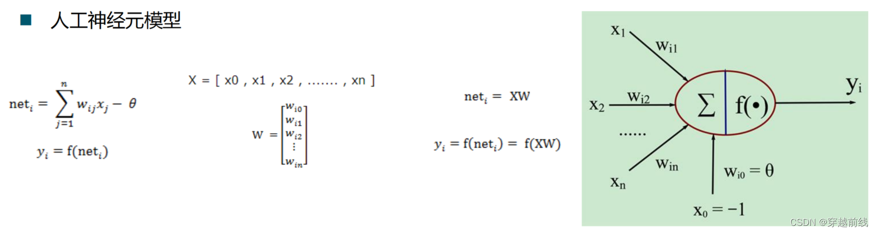
人工神经元模型
神经网络可以分为哪些?
- — 按照连接方式,可以分为:前向神经网络vs. 反馈(递归)神经网络
- — 按照学习方式,可以分为:有导师学习神经网络vs. 无导师学习神经网络
- — 按照实现功能,可以分为:拟合(回归)神经网络vs. 分类神经网络
BP神经网络概述
**Backpropagation **is a common method of teaching artificial neural networks how to perform a given task.
It is a **supervised learning **method, and is a generalization of the delta rule. It requires a teacher that knows, or can calculate, the desired output for any input in the training set.
Backpropagation requires that the **activation function **used by the artificial neurons (or "nodes") be differentiable.
BP神经网络两大步骤
** Phase 1: Propagation **
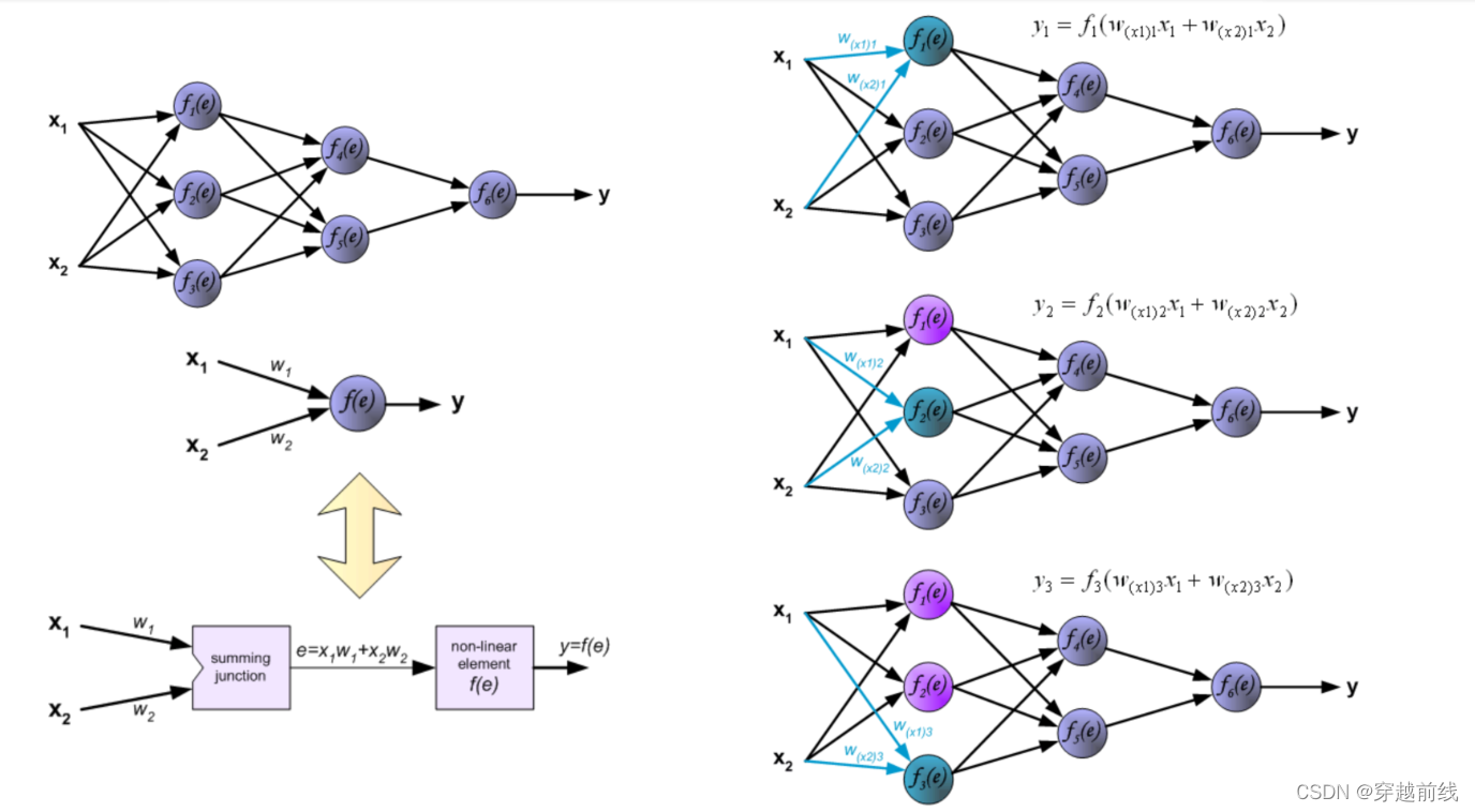
1. Forward propagation of a **training pattern’s input **through the neural network in order to generate the propagation’s output activations.
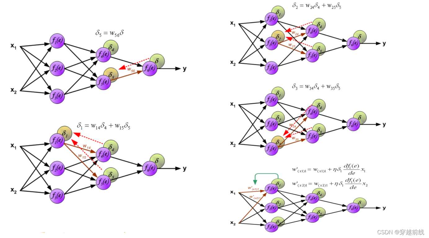
2. Back propagation of the **propagation’s output activations **through the neural network using the **training pattern’s ****target **in order to **generate the deltas **of all output and hidden neurons.
** Phase 2: Weight Update **
          1. Multiply its output delta and input activation to **get the gradient **of the weight.、

           2. Bring the weight in **the opposite direction **of the gradient by subtracting a ration of                       it from the weight.
BP神经网络图示

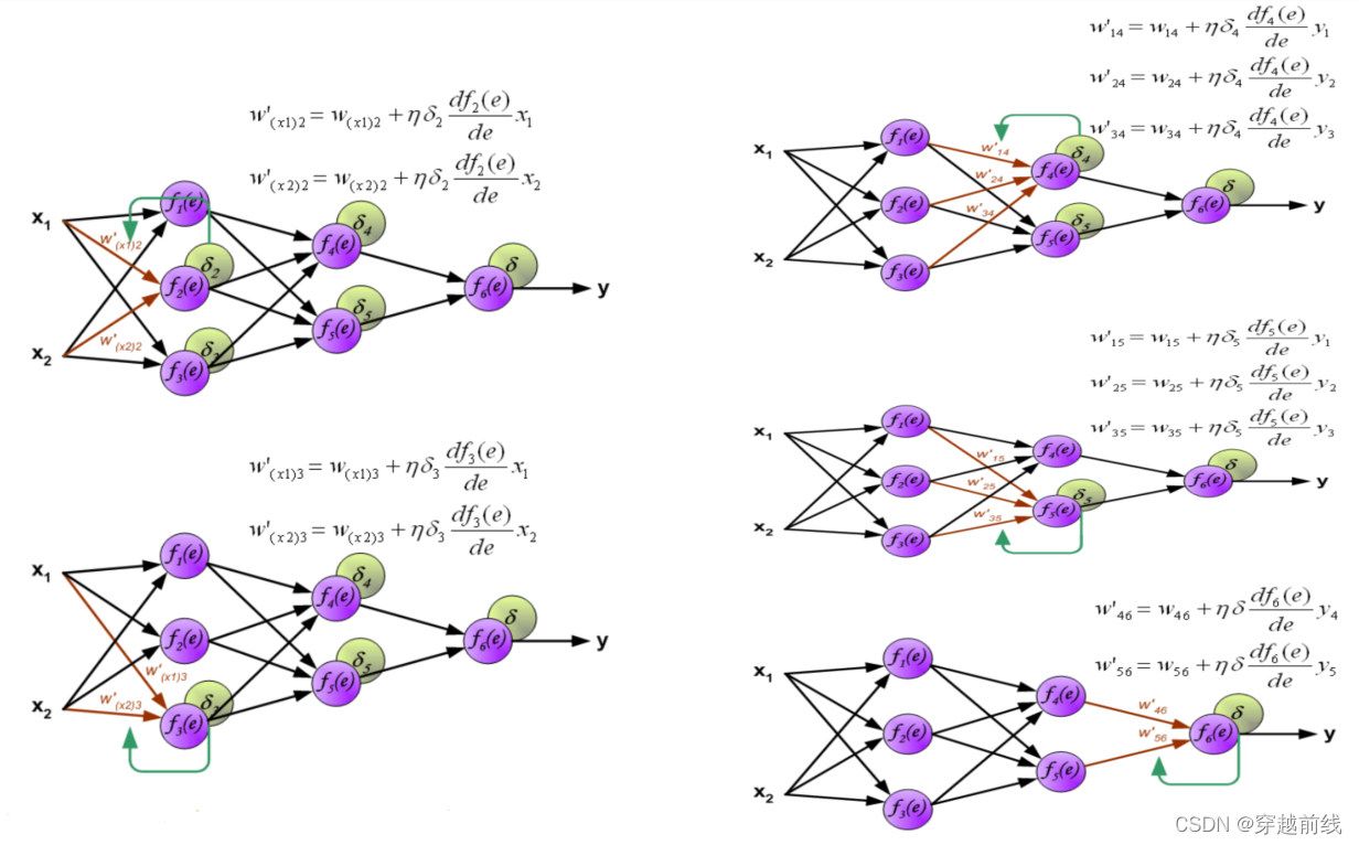
MATLAB实现所需掌握的知识
数据归一化
** 什么是归一化?**
** **将数据映射到[0, 1]或[-1, 1]区间或其他的区间
** 为什么要归一化?**** **
输入数据的单位不一样,有些数据的范围可能特别大,导致的结果是神经网络收敛慢、训练时间长。
数据范围大的输入在模式分类中的作用可能会偏大,而数据范围小的输入作用就可能会小。
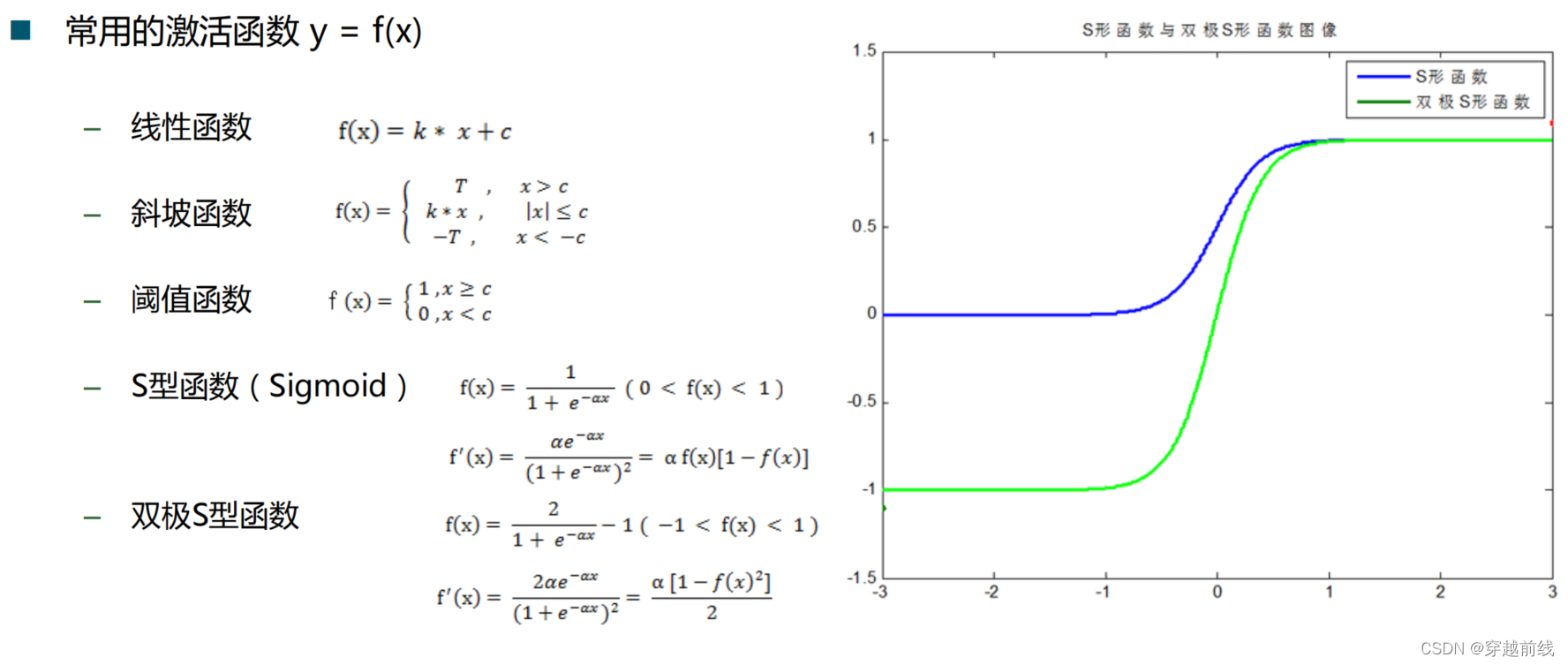
由于神经网络输出层的激活函数的值域是有限制的,因此需要将网络训练的目标数据映射到激活函数的值域。例如神经网络的输出层若采用S形激活 函数,由于S形函数的值域限制在(0,1),也就是说神经网络的输出只能限制在(0,1),所以训练数据的输出就要归一化到[0,1]区间。
S形激活函数在(0,1)区间以外区域很平缓,区分度太小。例如S形函数f(X)在参数a=1时,f(100)与f(5)只相差0.0067。
**归一化算法**
** ** 1. y = (x-min)/(max-min)
2. y = 2*(x-min)/(max-min)-1
常用重点函数
• mapminmax
    –      Process matrices by mapping row minimum and maximum values to [-1 1]

    –      [Y, PS] = mapminmax(X, YMIN, YMAX)

    –      Y = mapminmax('apply', X, PS)

    –      X = mapminmax('reverse', Y, PS)
• newff
    –      Create feed-forward backpropagation network

    –      net = newff(P, T, [S1 S2...S(N-l)], {TF1 TF2...TFNl}, BTF, BLF, PF, IPF, OPF, DDF)
• train
    –      Train neural network

    –      [net, tr, Y, E, Pf, Af] = train(net, P, T, Pi, Ai)
• sim
    –      Simulate neural network

    –      [Y, Pf, Af, E, perf] = sim(net, P, Pi, Ai, T)
BP神经网络MATLAB仿真过程
1. 清空环境变量
clear all
clc
2. 训练集/测试集的产生
2.1 导入数据
load spectra_data.mat
执行该程序,可以得到两个工作区变量
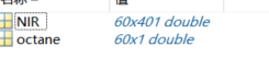
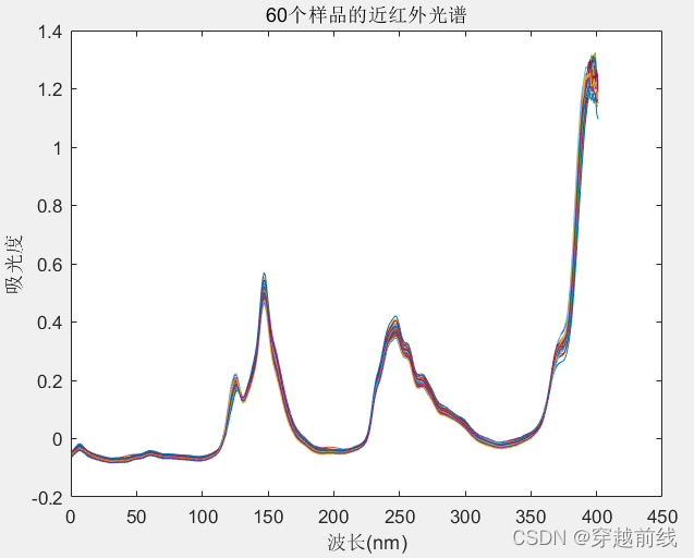
NIR是近红外光谱图原始数据,60代表着60个样品,使用plot(NIR')可以得到近红外光谱图
octane是结果,也就是目标值
2.2 随机产生训练集和测试集
训练集和测试集可以自行选择,也可以从原始数据中随机生成。本次实验中选择的是随机生成。
temp = randperm(size(NIR,1));
% 训练集--50个样本
P_train = NIR(temp(1:50),:)';        % '表示转置,使得 列 为样本的个数
T_train = octane(temp(1:50),:)';     % '特征与目标一定要保证列即样本个数相等
% 测试集--10个样本
P_test = NIR(temp(50:end),:)';       % '表示转置,使得 列 为样本的个数
T_test = octane(temp(50:end),:)';    % '特征与目标一定要保证列即样本个数相等
N = size(P_test,2);                  % 取出测试集样本的个数
3 数据归一化处理
对原始数据进行归一化处理,使其数据范围在0-1之间
[p_train, ps_input] = mapminmax(P_train,0,1); %调用归一化函数
p_test = mapminmax('apply',P_test,ps_input);

[t_train, ps_output] = mapminmax(T_train,0,1);
4. BP神经网络创建、训练及仿真测试
4.1 创建网络
使用newff函数便可以创建BP神经网络,其中参数9代表着神经元的个数
net = newff(p_train,t_train,9)  % 9代表神经元的个数
%view(net);                    % 使用view(net)可以看到BP神经网络的结构图
使用view(net)可以看到所创建的BP神经网络结构图
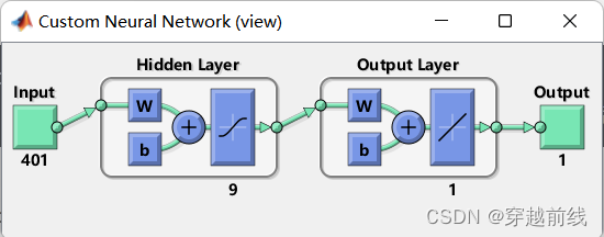
4.2 设置训练参数
net.trainParam.epochs = 1000    % 设置迭代次数
net.trainParam.goal = 1e-3;     % 设置训练目标,即误差精度
net.trainParam.lr = 0.01;       % 设置学习速率
4.3 训练网络
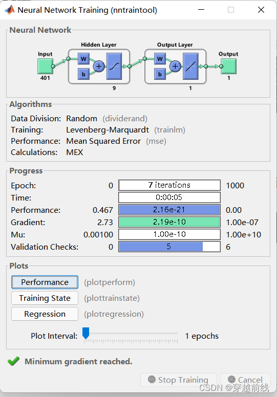
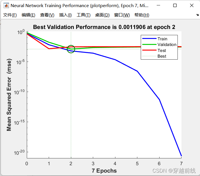
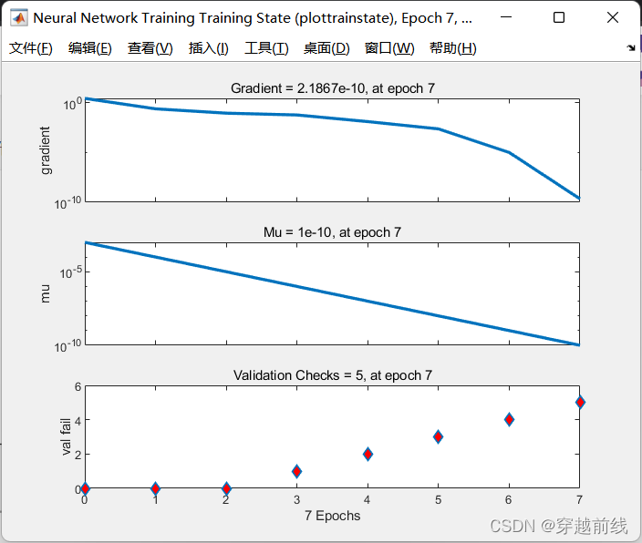
通过调用train函数便可以对神经网络进行训练
net = train(net,p_train,t_train);
运行代码,便可以看到训练指标和效果等等
4.4 仿真测试
将测试集输入sim预测函数,得到预测结果
t_sim = sim(net,p_test);
4.5 数据反归一化
此时的t_sim是归一化后的结果,为了与原数据进行对比,对t_sim进行反归一化。
T_sim = mapminmax('reverse',t_sim,ps_output); % T_sim为预测值
- 性能评价
预测结果效果如何,需要与真实结果对比,进行评估
5.1 相对误差error
error = abs(T_sim-T_test)./T_test;
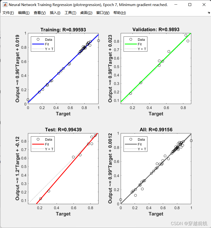
5.2 决定系数R^2
R2 = (N * sum(T_sim .* T_test) - sum(T_sim) * sum(T_test))^2 / ((N * sum((T_sim).^2) - (sum(T_sim))^2) * (N * sum((T_test).^2) - (sum(T_test))^2));
5.3 结果对比
result = [T_test' T_sim' error'];
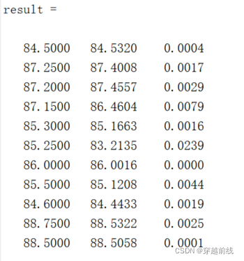
可以看到预测值与真实值基本一致,误差很小。
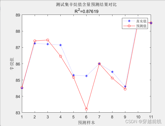
6. 绘图
figure
plot(1:N,T_test,'b:*',1:N,T_sim,'r-o')
legend('真实值','预测值')
xlabel('预测样本')
ylabel('辛烷值')
string = {'测试集辛烷值含量预测结果对比';['R^2=' num2str(R2)]};
title(string)
代码汇总如下
%% 1.清空环境变量
clear all
clc

%% 2.训练集/测试集产生
%% 2.1 导入数据
load spectra_data.mat
% plot(NIR');
% title('60个样品的近红外光谱');
% xlabel('波长(nm)');
% ylabel('吸光度');
%% 2.2 随机产生训练集和测试集
temp = randperm(size(NIR,1));
% 训练集--50个样本
P_train = NIR(temp(1:50),:)';        % '表示转置,使得 列 为样本的个数
T_train = octane(temp(1:50),:)';     % '特征与目标一定要保证列即样本个数相等
% 测试集--10个样本
P_test = NIR(temp(50:end),:)';       % '表示转置,使得 列 为样本的个数
T_test = octane(temp(50:end),:)';    % '特征与目标一定要保证列即样本个数相等
N = size(P_test,2);                  % 取出测试集样本的个数

%% 3 数据归一化
[p_train, ps_input] = mapminmax(P_train,0,1); %调用归一化函数
p_test = mapminmax('apply',P_test,ps_input);

[t_train, ps_output] = mapminmax(T_train,0,1);

%% 4. BP神经网络创建、训练及仿真测试
%% 4.1 创建网络
net = newff(p_train,t_train,9)  % 9代表神经元的个数
% view(net);                   % 使用view(net)可以看到BP神经网络的结构图

%% 4.2 设置训练参数
net.trainParam.epochs = 1000    % 设置迭代次数
net.trainParam.goal = 1e-3;     % 设置训练目标,即误差精度
net.trainParam.lr = 0.01;       % 设置学习速率

%% 4.3 训练网路
net = train(net,p_train,t_train);

%% 4.4 仿真测试
t_sim = sim(net,p_test);

%% 4.5 数据反归一化
T_sim = mapminmax('reverse',t_sim,ps_output); % T_sim为预测值

%% 5. 性能评价
%% 5.1 相对误差error
error = abs(T_sim-T_test)./T_test;

%% 5.2 决定系数R^2
R2 = (N * sum(T_sim .* T_test) - sum(T_sim) * sum(T_test))^2 / ((N * sum((T_sim).^2) - (sum(T_sim))^2) * (N * sum((T_test).^2) - (sum(T_test))^2));

%% 5.3 结果对比
result = [T_test' T_sim' error'];

%% 6. 绘图
figure
plot(1:N,T_test,'b:*',1:N,T_sim,'r-o')
legend('真实值','预测值')
xlabel('预测样本')
ylabel('辛烷值')
string = {'测试集辛烷值含量预测结果对比';['R^2=' num2str(R2)]};
title(string)
%%
版权归原作者 穿越前线 所有, 如有侵权,请联系我们删除。