
点击上方“Deephub Imba”,关注公众号,好文章不错过 !
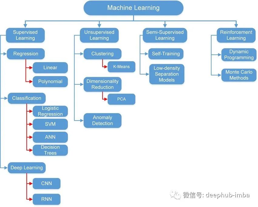
机器学习是人工智能的一门子科学,其中计算机和机器通常学会在没有人工干预或显式编程的情况下自行执行特定任务(当然,首先要对他们进行训练)。不同类型的机器学习技术可以划分到不同类别,如图 1 所示。方法的选择取决于问题的类型(分类、回归、聚类)、数据的类型(图像、图形、时间系列、音频等等)以及方法本身的配置(调优)。
在本文中,我们将使用 Python 中最著名的三个模块来实现一个简单的线性回归模型。使用 Python 的原因是它易于学习和应用。我们将使用的三个模块是:
1- Numpy:可以用于数组、矩阵、多维矩阵以及与它们相关的所有操作。
2- Keras:TensorFlow 的高级接口。它也用于支持和实现深度学习模型和浅层模型。它是由谷歌工程师开发的。
3- PyTorch:基于 Torch 的深度学习框架。它是由 Facebook 开发的。
所有这些模块都是开源的。Keras 和 PyTorch 都支持使用 GPU 来加快执行速度。
以下部分介绍线性回归的理论和概念。如果您已经熟悉理论并且想要实践部分,可以跳过到下一部分。
线性回归
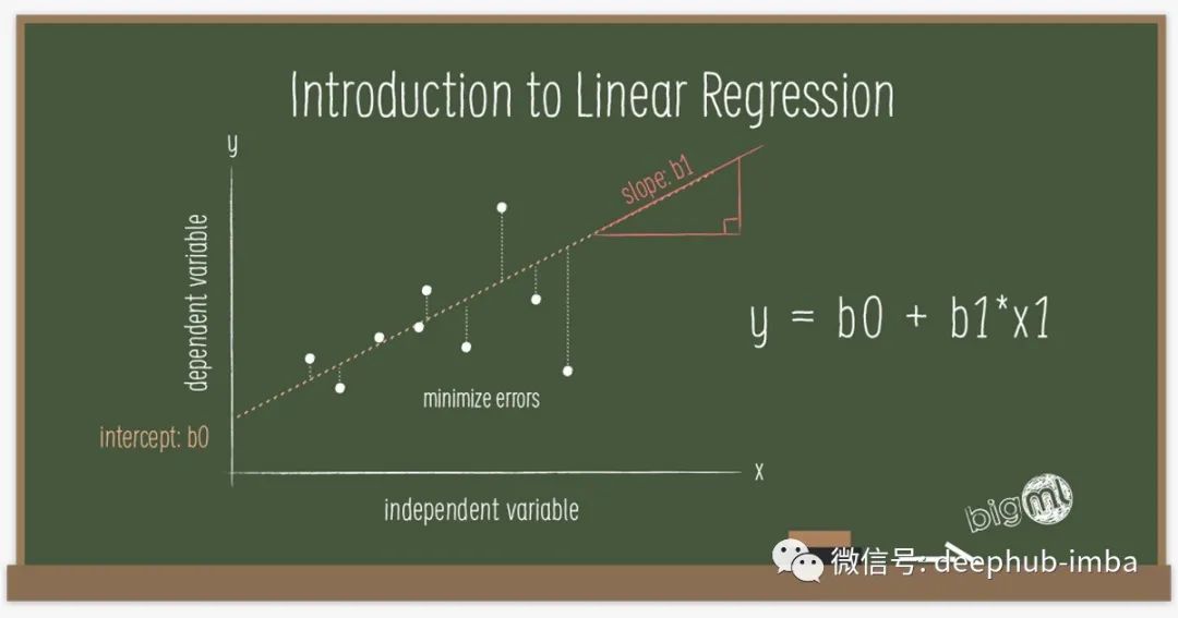
它是一种数学方法,可以将一条线与基础数据拟合。它假设输出和输入之间存在线性关系。输入称为特征或解释变量,输出称为目标或因变量。输出变量必须是连续的。例如,价格、速度、距离和温度。以下等式在数学上表示线性回归模型:
Y = W*X + B
如果把这个方程写成矩阵形式。Y 是输出矩阵,X 是输入矩阵,W 是权重矩阵,B 是偏置向量。权重和偏置是线性回归参数。有时权重和偏置分别称为斜率和截距。
训练该模型的第一步是随机初始化这些参数。然后它使用输入的数据来计算输出。通过测量误差将计算出的输出与实际输出进行比较,并相应地更新参数。并重复上述步骤。该误差称为 L2 范数(误差平方和),由下式给出:
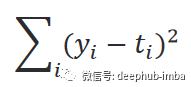
计算误差的函数又被称作损失函数,它可以有不同的公式。i 是数据样本数,y 是预测输出,t 是真实目标。根据以下等式中给出的梯度下降规则更新参数:
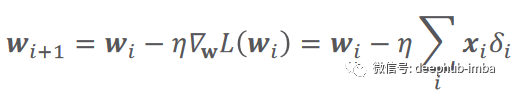
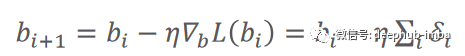
在这里,𝜂(希腊字母 eta)是学习率,它指定参数的更新步骤(更新速度)。𝛿(希腊字母 delta)只是预测输出和真实输出之间的差异。i 代表迭代(所谓的轮次)。𝛻 L(W) 是损失函数相对于权重的梯度(导数)。关于学习率的价值,有一点值得一提。较小的值会导致训练速度变慢,而较大的值会导致围绕局部最小值或发散(无法达到损失函数的局部最小值)的振荡。图 2 总结了以上所有内容。
现在让我们深入了解每个模块并将上面的方法实现。
Numpy 实现
我们将使用 Google Colab 作为我们的 IDE(集成开发环境),因为它功能强大,提供了所有必需的模块,无需安装(部分模块除外),并且可以免费使用。
为了简化实现,我们将考虑具有单个特征和偏置 (y = w1*x1 + b) 的线性关系。
让我们首先导入 Numpy 模块来实现线性回归模型和 Matplotlib 进行可视化。
# Numpy is needed to build the model
importnumpyasnp
# Import the module matplotlib for visualizing the data
importmatplotlib.pyplotasplt
我们需要一些数据来处理。数据由一个特征和一个输出组成。对于特征生成,我们将从随机均匀分布中生成 1000 个样本。
# We use this line to make the code reproducible (to get the same results when running)
np.random.seed(42)
# First, we should declare a variable containing the size of the training set we want to generate
observations = 1000

# Let us assume we have the following relationship
# y = 13x + 2
# y is the output and x is the input or feature
# We generate the feature randomly, drawing from an uniform distribution. There are 3 arguments of this method (low, high, size).
# The size of x is observations by 1. In this case: 1000 x 1.
x = np.random.uniform(low=-10, high=10, size=(observations,1))

# Let us print the shape of the feature vector
print (x.shape)
为了生成输出(目标),我们将使用以下关系:
Y = 13 * X + 2 + 噪声
这就是我们将尝试使用线性回归模型来估计的。权重值为 13,偏置为 2。噪声变量用于添加一些随机性。
np.random.seed(42)
# We add a small noise to our function for more randomness
noise = np.random.uniform(-1, 1, (observations,1))

# Produce the targets according to the f(x) = 13x + 2 + noise definition.
# This is a simple linear relationship with one weight and bias.
# In this way, we are basically saying: the weight is 13 and the bias is 2.
targets = 13*x+2+noise

# Check the shape of the targets just in case. It should be n x m, where n is the number of samples
# and m is the number of output variables, so 1000 x 1.
print (targets.shape)
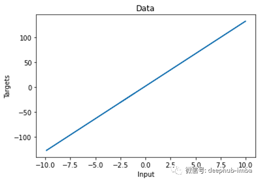
让我们绘制生成的数据。
# Plot x and targets
plt.plot(x,targets)

# Add labels to x axis and y axis
plt.ylabel('Targets')
plt.xlabel('Input')

# Add title to the graph
plt.title('Data')

# Show the plot
plt.show()
图 3 显示了这种线性关系:
对于模型训练,我们将从参数的一些初始值开始。它们是从给定范围内的随机均匀分布生成的。您可以看到这些值与真实值相差甚远。
np.random.seed(42)
# We will initialize the weights and biases randomly within a small initial range.
# init_range is the variable that will measure that.
init_range = 0.1

# Weights are of size k x m, where k is the number of input variables and m is the number of output variables
# In our case, the weights matrix is 1 x 1, since there is only one input (x) and one output (y)
weights = np.random.uniform(low=-init_range, high=init_range, size=(1, 1))

# Biases are of size 1 since there is only 1 output. The bias is a scalar.
biases = np.random.uniform(low=-init_range, high=init_range, size=1)

# Print the weights to get a sense of how they were initialized.
# You can see that they are far from the actual values.
print (weights)
print (biases)

[[-0.02509198]]
[0.09014286]
我们还为我们的训练设置了学习率。我们选择了 0.02 的值。这里可以通过尝试不同的值来探索性能。我们有了数据,初始化了参数,并设置了学习率,已准备好开始训练过程。我们通过将 epochs 设置为 100 来迭代数据。在每个 epoch 中,我们使用初始参数来计算新输出并将它们与实际输出进行比较。损失函数用于根据前面提到的梯度下降规则更新参数。新更新的参数用于下一次迭代。这个过程会不断重复,直到达到 epoch 数。可以有其他停止训练的标准,但我们今天不讨论它。
# Set some small learning rate
# 0.02 is going to work quite well for our example. Once again, you can play around with it.
# It is HIGHLY recommended that you play around with it.
learning_rate = 0.02

# We iterate over our training dataset 100 times. That works well with a learning rate of 0.02.
# We call these iteration epochs.
# Let us define a variable to store the loss of each epoch.
losses = []
foriinrange (100):

    # This is the linear model: y = xw + b equation
    outputs = np.dot(x,weights) +biases
    # The deltas are the differences between the outputs and the targets
    # Note that deltas here is a vector 1000 x 1
    deltas = outputs-targets

    # We are considering the L2-norm loss as our loss function (regression problem), but divided by 2.
    # Moreover, we further divide it by the number of observations to take the mean of the L2-norm.
    loss = np.sum(deltas**2) /2/observations

    # We print the loss function value at each step so we can observe whether it is decreasing as desired.
    print (loss)

    # Add the loss to the list
    losses.append(loss)

    # Another small trick is to scale the deltas the same way as the loss function
    # In this way our learning rate is independent of the number of samples (observations).
    # Again, this doesn't change anything in principle, it simply makes it easier to pick a single learning rate
    # that can remain the same if we change the number of training samples (observations).
    deltas_scaled = deltas/observations

    # Finally, we must apply the gradient descent update rules.
    # The weights are 1 x 1, learning rate is 1 x 1 (scalar), inputs are 1000 x 1, and deltas_scaled are 1000 x 1
    # We must transpose the inputs so that we get an allowed operation.
    weights = weights-learning_rate*np.dot(x.T,deltas_scaled)
    biases = biases-learning_rate*np.sum(deltas_scaled)

    # The weights are updated in a linear algebraic way (a matrix minus another matrix)
    # The biases, however, are just a single number here, so we must transform the deltas into a scalar.
    # The two lines are both consistent with the gradient descent methodology.
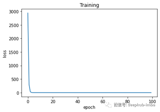
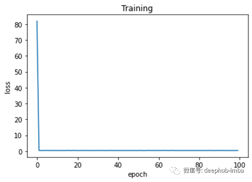
我们可以观察每个轮次的训练损失。
# Plot epochs and losses
plt.plot(range(100),losses)

# Add labels to x axis and y axis
plt.ylabel('loss')
plt.xlabel('epoch')

# Add title to the graph
plt.title('Training')

# Show the plot
# The curve is decreasing in each epoch, which is what we need
# After several epochs, we can see that the curve is flattened.
# This means the algorithm has converged and hence there are no significant updates
# or changes in the weights or biases.
plt.show()
正如我们从图 4 中看到的,损失在每个 epoch 中都在减少。这意味着模型越来越接近参数的真实值。几个 epoch 后,损失没有显着变化。这意味着模型已经收敛并且参数不再更新(或者更新非常小)。
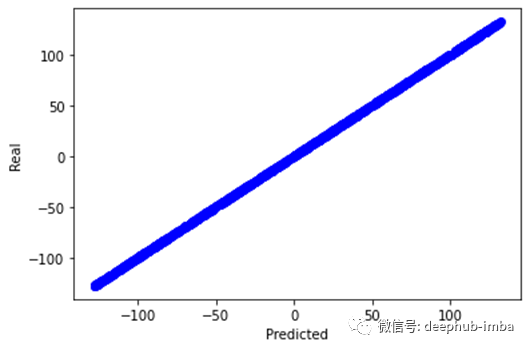
此外,我们可以通过绘制实际输出和预测输出来验证我们的模型在找到真实关系方面的指标。
# We print the real and predicted targets in order to see if they have a linear relationship.
# There is almost a total match between the real targets and predicted targets.
# This is a good signal of the success of our machine learning model.
plt.plot(outputs,targets, 'bo')
plt.xlabel('Predicted')
plt.ylabel('Real')
plt.show()

# We print the weights and the biases, so we can see if they have converged to what we wanted.
# We know that the real weight is 13 and the bias is 2
print (weights, biases)
这将生成如图 5 所示的图形。我们甚至可以打印最后一个 epoch 之后的参数值。显然,更新后的参数与实际参数非常接近。
[[13.09844702]] [1.73587336]
Numpy 实现线性回归模型就是这样。
Keras 实现
我们首先导入必要的模块。TensorFlow 是这个实现的核心。它是构建模型所必需的。Keras 是 TensorFlow 的抽象,以便于使用。
# Numpy is needed to generate the data
importnumpyasnp
# Matplotlib is needed for visualization
importmatplotlib.pyplotasplt
# TensorFlow is needed for model build
importtensorflowastf
为了生成数据(特征和目标),我们使用了 Numpy 中生成数据的代码。我们添加了一行来将 Numpy 数组保存在一个文件中,以防我们想将它们与其他模型一起使用(可能不需要,但添加它不会有什么坏处)。
np.savez('TF_intro', inputs=x, targets=targets)
Keras 有一个 Sequential 的类。它用于堆叠创建模型的层。由于我们只有一个特征和输出,因此我们将只有一个称为密集层的层。这一层负责线性变换 (W*X +B),这是我们想要的模型。该层有一个称为神经元的计算单元用于输出计算,因为它是一个回归模型。对于内核(权重)和偏置初始化,我们在给定范围内应用了均匀随机分布(与 Numpy 中相同,但是在层内指定)。
# Declare a variable where we will store the input size of our model
# It should be equal to the number of variables you have
input_size = 1
# Declare the output size of the model
# It should be equal to the number of outputs you've got (for regressions that's usually 1)
output_size = 1

# Outline the model
# We lay out the model in 'Sequential'
# Note that there are no calculations involved - we are just describing our network
model = tf.keras.Sequential([
                            # Each 'layer' is listed here
                            # The method 'Dense' indicates, our mathematical operation to be (xw + b)
                            tf.keras.layers.Input(shape=(input_size , )),
                            tf.keras.layers.Dense(output_size,
                                                 # there are extra arguments you can include to customize your model
                                                 # in our case we are just trying to create a solution that is
                                                 # as close as possible to our NumPy model
                                                 # kernel here is just another name for the weight parameter
                                                 kernel_initializer=tf.random_uniform_initializer(minval=-0.1, maxval=0.1),
                                                 bias_initializer=tf.random_uniform_initializer(minval=-0.1, maxval=0.1)
                                                 )
                            ])

# Print the structure of the model
model.summary()
为了训练模型,keras提供 fit 的方法可以完成这项工作。因此,我们首先加载数据,指定特征和标签,并设置轮次。在训练模型之前,我们通过选择合适的优化器和损失函数来配置模型。这就是 compile 的作用。我们使用了学习率为 0.02(与之前相同)的随机梯度下降,损失是均方误差。
# Load the training data from the NPZ
training_data = np.load('TF_intro.npz')

# We can also define a custom optimizer, where we can specify the learning rate
custom_optimizer = tf.keras.optimizers.SGD(learning_rate=0.02)

# 'compile' is the place where you select and indicate the optimizers and the loss
# Our loss here is the mean square error
model.compile(optimizer=custom_optimizer, loss='mse')

# finally we fit the model, indicating the inputs and targets
# if they are not otherwise specified the number of epochs will be 1 (a single epoch of training),
# so the number of epochs is 'kind of' mandatory, too
# we can play around with verbose; we prefer verbose=2
model.fit(training_data['inputs'], training_data['targets'], epochs=100, verbose=2)
我们可以在训练期间监控每个 epoch 的损失,看看是否一切正常。训练完成后,我们可以打印模型的参数。显然,模型已经收敛了与实际值非常接近的参数值。
# Extracting the weights and biases is achieved quite easily
model.layers[0].get_weights()

# We can save the weights and biases in separate variables for easier examination
# Note that there can be hundreds or thousands of them!
weights = model.layers[0].get_weights()[0]

bias = model.layers[0].get_weights()[1]
bias,weights

(array([1.9999999], dtype=float32), array([[13.1]], dtype=float32))
当您构建具有数千个参数和不同层的复杂模型时,TensorFlow 可以为您节省大量精力和代码行。由于模型太简单,这里并没有显示keras的优势。
PyTorch 实现
我们导入 Torch。这是必须的,因为它将用于创建模型。
# Numpy is needed for data generation
importnumpyasnp
# Pytorch is needed for model build
importtorch
数据生成部分未显示,因为它与前面使用的代码相同。但是Torch 只处理张量(torch.Tensor)。所以需要将特征和目标数组都转换为张量。最后,从这两个张量创建一个张量数据集。
# TensorDataset is needed to prepare the training data in form of tensors
fromtorch.utils.dataimportTensorDataset

# To run the model on either the CPU or GPU (if available)
device = 'cuda'iftorch.cuda.is_available() else'cpu'

# Since torch deals with tensors, we convert the numpy arrays into torch tensors
x_tensor = torch.from_numpy(x).float()
y_tensor = torch.from_numpy(targets).float()

# Combine the feature tensor and target tensor into torch dataset
train_data = TensorDataset(x_tensor , y_tensor)
模型的创建很简单。与keras类似,Sequential 类用于创建层堆栈。我们只有一个线性层(keras叫密集层),一个输入和一个输出。模型的参数使用定义的函数随机初始化。为了配置模型,我们设置了学习率、损失函数和优化器。还有其他参数需要设置,这里不做介绍。
# Initialize the seed to make the code reproducible
torch.manual_seed(42)

# This function is for model's parameters initialization
definit_weights(m):
    ifisinstance(m, torch.nn.Linear):
        torch.nn.init.uniform_(m.weight , a = -0.1 , b = 0.1)
        torch.nn.init.uniform_(m.bias , a = -0.1 , b = 0.1)

# Define the model using Sequential class
# It contains only a single linear layer with one input and one output
model = torch.nn.Sequential(torch.nn.Linear(1 , 1)).to(device)

# Initialize the model's parameters using the defined function from above
model.apply(init_weights)

# Print the model's parameters
print(model.state_dict())

# Specify the learning rate
lr = 0.02

# The loss function is the mean squared error
loss_fn = torch.nn.MSELoss(reduction = 'mean')

# The optimizer is the stochastic gradient descent with a certain learning rate
optimizer = torch.optim.SGD(model.parameters() , lr = lr)
我们将使用小批量梯度下降训练模型。DataLoader 负责从训练数据集创建批次。训练类似于keras的实现,但使用不同的语法。关于 Torch训练有几点补充:
1- 模型和批次必须在同一设备(CPU 或 GPU)上。
2- 模型必须设置为训练模式。
3- 始终记住在每个 epoch 之后将梯度归零以防止累积(对 epoch 的梯度求和),这会导致错误的值。
# DataLoader is needed for data batching
fromtorch.utils.dataimportDataLoader

# Training dataset is converted into batches of size 16 samples each.
# Shuffling is enabled for randomizing the data
train_loader = DataLoader(train_data , batch_size = 16 , shuffle = True)

# A function for training the model
# It is a function of a function (How fancy)
defmake_train_step(model , optimizer , loss_fn):
  deftrain_step(x , y):
    # Set the model to training mode
    model.train()
    # Feedforward the model with the data (features) to obtain the predictions
    yhat = model(x)
    # Calculate the loss based on the predicted and actual targets
    loss = loss_fn(y , yhat)
    # Perform the backpropagation to find the gradients
    loss.backward()
    # Update the parameters with the calculated gradients
    optimizer.step()
    # Set the gradients to zero to prevent accumulation
    optimizer.zero_grad()
    returnloss.item()
  returntrain_step

# Call the training function
train_step = make_train_step(model , optimizer , loss_fn)

# To store the loss of each epoch
losses = []

# Set the epochs to 100
epochs = 100

# Run the training function in each epoch on the batches of the data
# This is why we have two for loops
# Outer loop for epochs
# Inner loop for iterating through the training data batches
forepochinrange(epochs):
  # To accumulate the losses of all batches within a single epoch
  batch_loss = 0
  forx_batch , y_batchintrain_loader:
    x_batch = x_batch.to(device)
    y_batch = y_batch.to(device)
    loss = train_step(x_batch , y_batch)
    batch_loss = batch_loss+loss
  # 63 is not a magic number. It is the number of batches in the training set
  # we have 1000 samples and the batch size is 16 (defined in the DataLoader)
  # 1000/16 = 63
  epoch_loss = batch_loss/63
  losses.append(epoch_loss)

# Print the parameters after the training is done
print(model.state_dict())

OrderedDict([('0.weight', tensor([[13.0287]], device='cuda:0')), ('0.bias', tensor([2.0096], device='cuda:0'))])
作为最后一步,我们可以绘制 epoch 上的训练损失以观察模型的性能。如图 6 所示。
完成。让我们总结一下到目前为止我们学到的东西。
总结
线性回归被认为是最容易实现和解释的机器学习模型之一。 在本文中,我们使用 Python 中的三个不同的流行模块实现了线性回归。还有其他模块可用于创建。例如:Scikitlearn。本文的代码在这里可以找到:https://github.com/Motamensalih/Simple-Linear-Regression
作者:Motamen MohammedAhmed
喜欢就关注一下吧:
 点个 在看 你最好看!********** **********