聚类算法（上）：8个常见的无监督聚类方法介绍和比较

无监督聚类方法的评价指标必须依赖于数据和聚类结果的内在属性，例如聚类的紧凑性和分离性，与外部知识的一致性，以及同一算法不同运行结果的稳定性。

本文将全面概述Scikit-Learn库中用于的聚类技术以及各种评估方法。

本文将分为2个部分，1、常见算法比较 2、聚类技术的各种评估方法

本文作为第一部分将介绍和比较各种聚类算法：

• K-Means
• Affinity Propagation
• Agglomerative Clustering
• Mean Shift Clustering
• Bisecting K-Means
• DBSCAN
• OPTICS
• BIRCH

首先我们生成一些数据，后面将使用这些数据作为聚类技术的输入。

 importpandasaspd
 importnumpyasnp
 importseabornassns
 importmatplotlib.pyplotasplt
 
 #Set the number of samples and features
 n_samples=1000
 n_features=4
 
 #Create an empty array to store the data
 data=np.empty((n_samples, n_features))
 
 #Generate random data for each feature
 foriinrange(n_features):
   data[:, i] =np.random.normal(size=n_samples)
 
 #Create 5 clusters with different densities and centroids
 cluster1=data[:200, :] +np.random.normal(size=(200, n_features), scale=0.5)
 cluster2=data[200:400, :] +np.random.normal(size=(200, n_features), scale=1) +np.array([5,5,5,5])
 cluster3=data[400:600, :] +np.random.normal(size=(200, n_features), scale=1.5) +np.array([-5,-5,-5,-5])
 cluster4=data[600:800, :] +np.random.normal(size=(200, n_features), scale=2) +np.array([5,-5,5,-5])
 cluster5=data[800:, :] +np.random.normal(size=(200, n_features), scale=2.5) +np.array([-5,5,-5,5])
 
 #Combine the clusters into one dataset
 X=np.concatenate((cluster1, cluster2, cluster3, cluster4, cluster5))
 
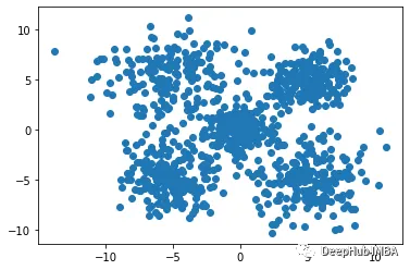
 # Plot the data
 plt.scatter(X[:, 0], X[:, 1])
 plt.show()

结果如下：

我们将用特征值和簇ID创建一个DF。稍后在模型性能时将使用这些数据。

 df=pd.DataFrame(X, columns=["feature_1", "feature_2", "feature_3", "feature_4"])
 cluster_id=np.concatenate((np.zeros(200), np.ones(200), np.full(200, 2), np.full(200, 3), np.full(200, 4)))
 df["cluster_id"] =cluster_id
 df

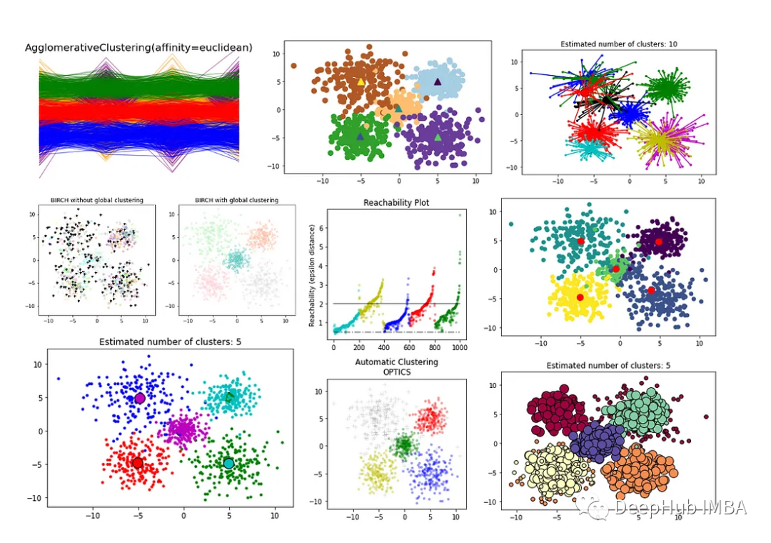
现在我们将构建和可视化8个不同的聚类模型:

1、K-Means

K-Means聚类算法是一种常用的聚类算法，它将数据点分为K个簇，每个簇的中心点是其所有成员的平均值。K-Means算法的核心是迭代寻找最优的簇心位置，直到达到收敛状态。

K-Means算法的优点是简单易懂，计算速度较快，适用于大规模数据集。但是它也存在一些缺点，例如对于非球形簇的处理能力较差，容易受到初始簇心的选择影响，需要预先指定簇的数量K等。此外，当数据点之间存在噪声或者离群点时，K-Means算法可能会将它们分配到错误的簇中。

 #K-Means
 fromsklearn.clusterimportKMeans
 
 #Define function:
 kmeans=KMeans(n_clusters=5)
 
 #Fit the model:
 km=kmeans.fit(X)
 km_labels=km.labels_
 
 #Print results:
 #print(kmeans.labels_)
 
 #Visualise results:
 plt.scatter(X[:, 0], X[:, 1], 
             c=kmeans.labels_,      
             s=70, cmap='Paired')
 plt.scatter(kmeans.cluster_centers_[:, 0],
             kmeans.cluster_centers_[:, 1],
             marker='^', s=100, linewidth=2, 
             c=[0, 1, 2, 3, 4])

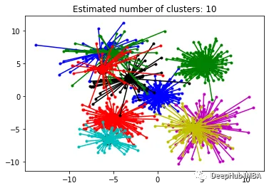
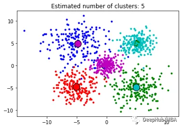
2、Affinity Propagation

Affinity Propagation是一种基于图论的聚类算法，旨在识别数据中的"exemplars"(代表点)和"clusters"(簇)。与K-Means等传统聚类算法不同，Affinity Propagation不需要事先指定聚类数目，也不需要随机初始化簇心，而是通过计算数据点之间的相似性得出最终的聚类结果。

Affinity Propagation算法的优点是不需要预先指定聚类数目，且能够处理非凸形状的簇。但是该算法的计算复杂度较高，需要大量的存储空间和计算资源，并且对于噪声点和离群点的处理能力较弱。

 fromsklearn.clusterimportAffinityPropagation
 
 #Fit the model:
 af=AffinityPropagation(preference=-563, random_state=0).fit(X)
 cluster_centers_indices=af.cluster_centers_indices_
 af_labels=af.labels_
 n_clusters_=len(cluster_centers_indices)
 
 #Print number of clusters:
 print(n_clusters_)
 
 importmatplotlib.pyplotasplt
 fromitertoolsimportcycle
 
 plt.close("all")
 plt.figure(1)
 plt.clf()
 
 colors=cycle("bgrcmykbgrcmykbgrcmykbgrcmyk")
 fork, colinzip(range(n_clusters_), colors):
     class_members=af_labels==k
     cluster_center=X[cluster_centers_indices[k]]
     plt.plot(X[class_members, 0], X[class_members, 1], col+".")
     plt.plot(
         cluster_center[0],
         cluster_center[1],
         "o",
         markerfacecolor=col,
         markeredgecolor="k",
         markersize=14,
     )
     forxinX[class_members]:
         plt.plot([cluster_center[0], x[0]], [cluster_center[1], x[1]], col)
 
 plt.title("Estimated number of clusters: %d"%n_clusters_)
 plt.show()

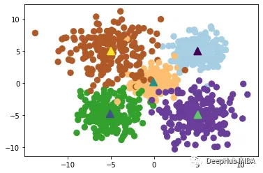
3、Agglomerative Clustering

凝聚层次聚类（Agglomerative Clustering）是一种自底向上的聚类算法，它将每个数据点视为一个初始簇，并将它们逐步合并成更大的簇，直到达到停止条件为止。在该算法中，每个数据点最初被视为一个单独的簇，然后逐步合并簇，直到所有数据点被合并为一个大簇。

Agglomerative Clustering算法的优点是适用于不同形状和大小的簇，且不需要事先指定聚类数目。此外，该算法也可以输出聚类层次结构，便于分析和可视化。缺点是计算复杂度较高，尤其是在处理大规模数据集时，需要消耗大量的计算资源和存储空间。此外，该算法对初始簇的选择也比较敏感，可能会导致不同的聚类结果。

 fromsklearn.clusterimportAgglomerativeClustering
 
 #Fit the model:
 clustering=AgglomerativeClustering(n_clusters=5).fit(X)
 
 AC_labels=clustering.labels_
 n_clusters=clustering.n_clusters_
 
 print("number of estimated clusters : %d"%clustering.n_clusters_)
 
 # Plot clustering results
 colors= ['purple', 'orange', 'green', 'blue', 'red']
 
 forindex, metricinenumerate([#"cosine", 
                                 "euclidean", 
                                 #"cityblock"
                                 ]):
     model=AgglomerativeClustering(
         n_clusters=5, linkage="ward", affinity=metric
     )
     model.fit(X)
     plt.figure()
     plt.axes([0, 0, 1, 1])
     forl, cinzip(np.arange(model.n_clusters), colors):
         plt.plot(X[model.labels_==l].T, c=c, alpha=0.5)
     plt.axis("tight")
     plt.axis("off")
     plt.suptitle("AgglomerativeClustering(affinity=%s)"%metric, size=20)
 
 
 plt.show()

4、Mean Shift Clustering

Mean Shift Clustering是一种基于密度的非参数聚类算法，其基本思想是通过寻找数据点密度最大的位置（称为"局部最大值"或"高峰"），来识别数据中的簇。算法的核心是通过对每个数据点进行局部密度估计，并将密度估计的结果用于计算数据点移动的方向和距离。算法的核心是通过对每个数据点进行局部密度估计，并将密度估计的结果用于计算数据点移动的方向和距离。

Mean Shift Clustering算法的优点是不需要指定簇的数目，且对于形状复杂的簇也有很好的效果。算法还能够有效地处理噪声数据。他的缺点也是计算复杂度较高，尤其是在处理大规模数据集时，需要消耗大量的计算资源和存储空间，该算法还对初始参数的选择比较敏感，需要进行参数调整和优化。

 fromsklearn.clusterimportMeanShift, estimate_bandwidth
 
 # The following bandwidth can be automatically detected using
 bandwidth=estimate_bandwidth(X, quantile=0.2, n_samples=100)
 
 #Fit the model:
 ms=MeanShift(bandwidth=bandwidth)
 ms.fit(X)
 MS_labels=ms.labels_
 cluster_centers=ms.cluster_centers_
 
 labels_unique=np.unique(labels)
 n_clusters_=len(labels_unique)
 
 print("number of estimated clusters : %d"%n_clusters_)
 
 fromitertoolsimportcycle
 
 plt.figure(1)
 plt.clf()
 
 colors=cycle("bgrcmykbgrcmykbgrcmykbgrcmyk")
 fork, colinzip(range(n_clusters_), colors):
     my_members=labels==k
     cluster_center=cluster_centers[k]
     plt.plot(X[my_members, 0], X[my_members, 1], col+".")
     plt.plot(
         cluster_center[0],
         cluster_center[1],
         "o",
         markerfacecolor=col,
         markeredgecolor="k",
         markersize=14,
     )
 plt.title("Estimated number of clusters: %d"%n_clusters_)
 plt.show()

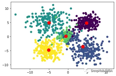
5、Bisecting K-Means

Bisecting K-Means是一种基于K-Means算法的层次聚类算法，其基本思想是将所有数据点划分为一个簇，然后将该簇分成两个子簇，并对每个子簇分别应用K-Means算法，重复执行这个过程，直到达到预定的聚类数目为止。

算法首先将所有数据点视为一个初始簇，然后对该簇应用K-Means算法，将该簇分成两个子簇，并计算每个子簇的误差平方和（SSE）。然后，选择误差平方和最大的子簇，并将其再次分成两个子簇，重复执行这个过程，直到达到预定的聚类数目为止。

Bisecting K-Means算法的优点是具有较高的准确性和稳定性，能够有效地处理大规模数据集，并且不需要指定初始聚类数目。该算法还能够输出聚类层次结构，便于分析和可视化。缺点是计算复杂度较高，尤其是在处理大规模数据集时，需要消耗大量的计算资源和存储空间。此外该算法对初始簇的选择也比较敏感，可能会导致不同的聚类结果。

 fromsklearn.clusterimportBisectingKMeans
 
 #Build and fit model:
 bisect_means=BisectingKMeans(n_clusters=5).fit(X)
 BKM_labels=bisect_means.labels_
 
 #Print model attributes:
 #print('Labels: ', bisect_means.labels_)
 print('Number of clusters: ', bisect_means.n_clusters)
 
 #Define varaibles to be included in scatterdot:
 y=bisect_means.labels_
 #print(y)
 centers=bisect_means.cluster_centers_
 
 # Visualize the results using a scatter plot
 plt.scatter(X[:, 0], X[:, 1], c=y)
 plt.scatter(centers[:, 0], centers[:, 1], c='r', s=100)
 
 plt.show()

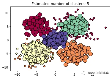
6、DBSCAN

DBSCAN (Density-Based Spatial Clustering of Applications with Noise)是一种基于密度的聚类算法，其可以有效地发现任意形状的簇，并能够处理噪声数据。DBSCAN算法的核心思想是：对于一个给定的数据点，如果它的密度达到一定的阈值，则它属于一个簇中；否则，它被视为噪声点。

DBSCAN算法的优点是能够自动识别簇的数目，并且对于任意形状的簇都有较好的效果。并且还能够有效地处理噪声数据，不需要预先指定簇的数目。缺点是对于密度差异较大的数据集，可能会导致聚类效果不佳，需要进行参数调整和优化。另外该算法对于高维数据集的效果也不如其他算法

 fromsklearn.clusterimportDBSCAN
 
 db=DBSCAN(eps=3, min_samples=10).fit(X)
 DBSCAN_labels=db.labels_
 
 # Number of clusters in labels, ignoring noise if present.
 n_clusters_=len(set(labels)) - (1if-1inlabelselse0)
 n_noise_=list(labels).count(-1)
 
 print("Estimated number of clusters: %d"%n_clusters_)
 print("Estimated number of noise points: %d"%n_noise_)
 
 unique_labels=set(labels)
 core_samples_mask=np.zeros_like(labels, dtype=bool)
 core_samples_mask[db.core_sample_indices_] =True
 
 colors= [plt.cm.Spectral(each) foreachinnp.linspace(0, 1, len(unique_labels))]
 fork, colinzip(unique_labels, colors):
     ifk==-1:
         # Black used for noise.
         col= [0, 0, 0, 1]
 
     class_member_mask=labels==k
 
     xy=X[class_member_mask&core_samples_mask]
     plt.plot(
         xy[:, 0],
         xy[:, 1],
         "o",
         markerfacecolor=tuple(col),
         markeredgecolor="k",
         markersize=14,
     )
 
     xy=X[class_member_mask&~core_samples_mask]
     plt.plot(
         xy[:, -1],
         xy[:, 1],
         "o",
         markerfacecolor=tuple(col),
         markeredgecolor="k",
         markersize=6,
     )
 
 plt.title(f"Estimated number of clusters: {n_clusters_}")
 plt.show()

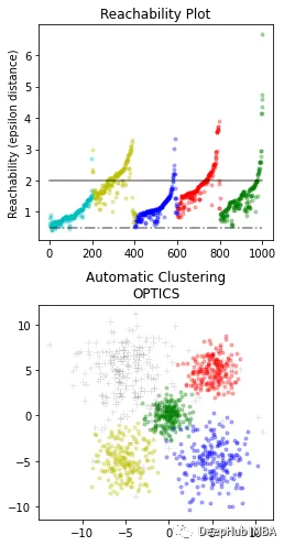
7、OPTICS

OPTICS（Ordering Points To Identify the Clustering Structure）是一种基于密度的聚类算法，其能够自动确定簇的数量，同时也可以发现任意形状的簇，并能够处理噪声数据。OPTICS算法的核心思想是：对于一个给定的数据点，通过计算它到其它点的距离，确定其在密度上的可达性，从而构建一个基于密度的距离图。然后，通过扫描该距离图，自动确定簇的数量，并对每个簇进行划分。

OPTICS算法的优点是能够自动确定簇的数量，并能够处理任意形状的簇，并能够有效地处理噪声数据。该算法还能够输出聚类层次结构，便于分析和可视化。缺点是计算复杂度较高，尤其是在处理大规模数据集时，需要消耗大量的计算资源和存储空间。另外就是该算法对于密度差异较大的数据集，可能会导致聚类效果不佳。

 fromsklearn.clusterimportOPTICS
 importmatplotlib.gridspecasgridspec
 
 #Build OPTICS model:
 clust=OPTICS(min_samples=3, min_cluster_size=100, metric='euclidean')
 
 # Run the fit
 clust.fit(X)
 
 space=np.arange(len(X))
 reachability=clust.reachability_[clust.ordering_]
 OPTICS_labels=clust.labels_[clust.ordering_]
 labels=clust.labels_[clust.ordering_]
 
 plt.figure(figsize=(10, 7))
 G=gridspec.GridSpec(2, 3)
 ax1=plt.subplot(G[0, 0])
 ax2=plt.subplot(G[1, 0])
 
 
 # Reachability plot
 colors= ["g.", "r.", "b.", "y.", "c."]
 forklass, colorinzip(range(0, 5), colors):
     Xk=space[labels==klass]
     Rk=reachability[labels==klass]
     ax1.plot(Xk, Rk, color, alpha=0.3)
 ax1.plot(space[labels==-1], reachability[labels==-1], "k.", alpha=0.3)
 ax1.set_ylabel("Reachability (epsilon distance)")
 ax1.set_title("Reachability Plot")
 
 # OPTICS
 colors= ["g.", "r.", "b.", "y.", "c."]
 forklass, colorinzip(range(0, 5), colors):
     Xk=X[clust.labels_==klass]
     ax2.plot(Xk[:, 0], Xk[:, 1], color, alpha=0.3)
 ax2.plot(X[clust.labels_==-1, 0], X[clust.labels_==-1, 1], "k+", alpha=0.1)
 ax2.set_title("Automatic Clustering\nOPTICS")
 
 
 plt.tight_layout()
 plt.show()

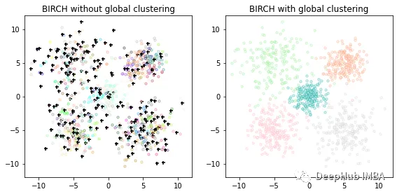
8、BIRCH

BIRCH（Balanced Iterative Reducing and Clustering using Hierarchies）是一种基于层次聚类的聚类算法，其可以快速地处理大规模数据集，并且对于任意形状的簇都有较好的效果。BIRCH算法的核心思想是：通过对数据集进行分级聚类，逐步减小数据规模，最终得到簇结构。BIRCH算法采用一种类似于B树的结构，称为CF树，它可以快速地插入和删除子簇，并且可以自动平衡，从而确保簇的质量和效率。

BIRCH算法的优点是能够快速处理大规模数据集，并且对于任意形状的簇都有较好的效果。该算法对于噪声数据和离群点也有较好的容错性。缺点是对于密度差异较大的数据集，可能会导致聚类效果不佳，对于高维数据集的效果也不如其他算法。

 importmatplotlib.colorsascolors
 fromsklearn.clusterimportBirch, MiniBatchKMeans
 fromtimeimporttime
 fromitertoolsimportcycle
 
 # Use all colors that matplotlib provides by default.
 colors_=cycle(colors.cnames.keys())
 
 fig=plt.figure(figsize=(12, 4))
 fig.subplots_adjust(left=0.04, right=0.98, bottom=0.1, top=0.9)
 
 # Compute clustering with BIRCH with and without the final clustering step
 # and plot.
 birch_models= [
     Birch(threshold=1.7, n_clusters=None),
     Birch(threshold=1.7, n_clusters=5),
 ]
 final_step= ["without global clustering", "with global clustering"]
 
 
 forind, (birch_model, info) inenumerate(zip(birch_models, final_step)):
     t=time()
     birch_model.fit(X)
     print("BIRCH %s as the final step took %0.2f seconds"% (info, (time() -t)))
 
     # Plot result
     labels=birch_model.labels_
     centroids=birch_model.subcluster_centers_
     n_clusters=np.unique(labels).size
     print("n_clusters : %d"%n_clusters)
 
     ax=fig.add_subplot(1, 3, ind+1)
     forthis_centroid, k, colinzip(centroids, range(n_clusters), colors_):
         mask=labels==k
         ax.scatter(X[mask, 0], X[mask, 1], c="w", edgecolor=col, marker=".", alpha=0.5)
         ifbirch_model.n_clustersisNone:
             ax.scatter(this_centroid[0], this_centroid[1], marker="+", c="k", s=25)
     ax.set_ylim([-12, 12])
     ax.set_xlim([-12, 12])
     ax.set_autoscaley_on(False)
     ax.set_title("BIRCH %s"%info)
 
 plt.show()

总结

上面就是我们常见的8个聚类算法，我们对他们进行了简单的说明和比较，并且用sklearn演示了如何使用，在下一篇文章中我们将介绍聚类模型评价方法。