
使用Python根据汇总统计信息添加新特性,本文将告诉你如何计算几个时间序列中的滚动统计信息。将这些信息添加到解释变量中通常会获得更好的预测性能。
简介
自回归
多变量时间序列包含两个或多个变量,研究这些数据集的目的是预测一个或多个变量,参见下面的示例。
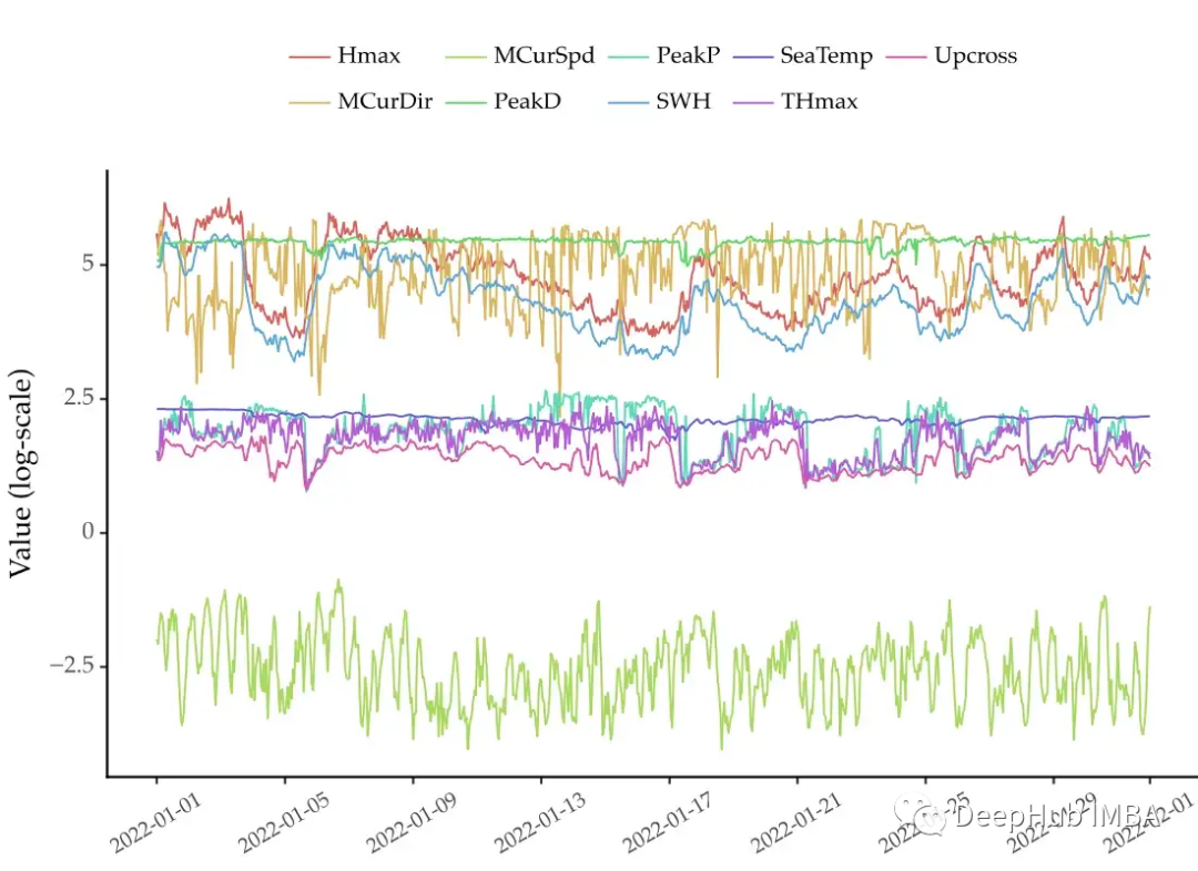
上图是包含9个变量的多变量时间序列。这些是智能浮标捕捉到的海洋状况。
大多数预测模型都是基于自回归的。这相当于解决了一个监督学习回归任务。该序列的未来值是目标变量。输入的解释变量是每个变量最近的过去值。
自回归在一个主要假设下工作。最近的过去值包含了关于未来的足够信息。但这可能不一定是真的。我们可以尝试从最近的数据中提取更多的信息。例如,滚动汇总统计信息有助于描述最近的动态。
自动化特征工程
特征工程包括提取和生成解释变量,这是任何数据科学项目的关键。特征的质量是模型性能的一个核心方面,所以数据科学家在这个过程中花费了大量的时间。
特性工程通常是一个特别的过程:数据科学家基于他们的领域知识和专业知识创建特性,如果该过程的能够自动化化处理将会为我们节省很多的时间。让我们看看如何在多元时间序列中做到这一点。
基线模型
读取数据
我们将使用从智能浮标收集的多元时间序列作为本文的数据集 [1]。 这个浮标位于爱尔兰海岸。 它捕获了 9 个与海洋条件相关的变量。 其中包括海水温度、波浪高度和海水流速等。 上面的图 1 显示了 2022 年第一个月的情况。
以下是使用 pandas 读取这些数据的方法:
 import pandas as pd

 # skipping second row, setting time column as a datetime column
 # dataset available here: https://github.com/vcerqueira/blog/tree/main/data
 buoy = pd.read_csv('data/smart_buoy.csv',
                    skiprows=[1],
                    parse_dates=['time'])

 # setting time as index
 buoy.set_index('time', inplace=True)
 # resampling to hourly data
 buoy = buoy.resample('H').mean()
 # simplifying column names
 buoy.columns = [
     'PeakP', 'PeakD', 'Upcross',
     'SWH', 'SeaTemp', 'Hmax', 'THmax',
     'MCurDir', 'MCurSpd'
 ]
这个数据集研究的目标是预测SWH(显著波高)变量的未来值。这个变量常被用来量化海浪的高度。这个问题的一个用例是估计海浪发电的大小,因为这种能源是一种越来越受欢迎的替代不可再生能源。
自回归模型
时间序列是多元的,所以可以使用ARDL(Auto-regressive distributed lags)方法来解决这个任务。我们在之前也介绍过则个方法。下面是这个方法的实现:
 import pandas as pd

 from sklearn.model_selection import train_test_split
 from sklearn.metrics import mean_absolute_percentage_error as mape
 from sklearn.multioutput import MultiOutputRegressor
 from lightgbm import LGBMRegressor

 # https://github.com/vcerqueira/blog/blob/main/src/tde.py
 from src.tde import time_delay_embedding

 target_var = 'SWH'

 colnames = buoy.columns.tolist()

 # create data set with lagged features using time delay embedding
 buoy_ds = []
 for col in buoy:
     col_df = time_delay_embedding(buoy[col], n_lags=24, horizon=12)
     buoy_ds.append(col_df)

 # concatenating all variables
 buoy_df = pd.concat(buoy_ds, axis=1).dropna()

 # defining target (Y) and explanatory variables (X)
 predictor_variables = buoy_df.columns.str.contains('\(t\-')
 target_variables = buoy_df.columns.str.contains(f'{target_var}\(t\+')
 X = buoy_df.iloc[:, predictor_variables]
 Y = buoy_df.iloc[:, target_variables]

 # train/test split
 X_tr, X_ts, Y_tr, Y_ts = train_test_split(X, Y, test_size=0.3, shuffle=False)

 # fitting a lgbm model without feature engineering
 model_wo_fe = MultiOutputRegressor(LGBMRegressor())
 model_wo_fe.fit(X_tr, Y_tr)

 # getting forecasts for the test set
 preds_wo_fe = model_wo_fe.predict(X_ts)

 # computing the MAPE error
 mape(Y_ts, preds_wo_fe)
 # 0.238
首先将时间序列转化为一个自回归问题。这是通过函数time_delay_embedding完成的。预测的目标是预测未来12个SWH值(horizon=12)。解释变量是序列中每个变量的过去的24个值(n_lag =24)。
我们这里直接使用LightGBM对每个预测层位进行训练。这种方法法是一种常用的多步超前预测方法。它在scikit-learn中也有实现,名为MultiOutputRegressor。
上面的代码构建和测试一个自回归模型。解释变量只包括每个变量最近的过去值。结果的平均绝对百分比误差为0.238。
我们把这个结果作为基类对比,让我们看看是否可以通过特性工程来提高。
多元时间序列的特征工程
本文本将介绍两种从多元时间序列中提取特征的方法:
- 单变量特征提取。计算各变量的滚动统计。例如,滚动平均可以用来消除虚假的观测;
- 二元特征提取。计算变量对的滚动统计,以总结它们的相互作用。例如,两个变量之间的滚动协方差。
单变量特征提取
我们可以总结每个变量最近的过去值。例如,计算滚动平均来总结最近的情况。或者滚动差量来了解最近的分散程度。
 import numpy as np

 SUMMARY_STATS = {
     'mean': np.mean,
     'sdev': np.std,
 }

 univariate_features = {}
 # for each column in the data
 for col in colnames:
     # get lags for that column
     X_col = X.iloc[:, X.columns.str.startswith(col)]

     # for each summary stat
     for feat, func in SUMMARY_STATS.items():
         # compute that stat along the rows
         univariate_features[f'{col}_{feat}'] = X_col.apply(func, axis=1)

 # concatenate features into a pd.DF
 univariate_features_df = pd.concat(univariate_features, axis=1)
如果能需要添加更多的统计数据。可以向SUMMARY_STATS字典添加函数来实现这一点。将这些函数放在一个字典中可以保持代码整洁。
二元特征提取
单变量统计漏掉了不同变量之间潜在的相互作用。所以我们可以使用二元特征提取过程捕获这些信息。
这个想法是为不同的变量对计算特征。可以使用二元统计总结了这些对的联合动态。
有两种方法可以做到这一点:
- 滚动二元统计。计算以变量对作为输入的统计信息。例如,滚动协方差或滚动相关性滚动二元统计的例子包括协方差、相关性或相对熵。
- 滚动二元变换,然后单变量统计。这将一对变量转换为一个变量,并对该变量进行统计。例如,计算元素相互关系,然后取其平均值。有许多二元转换的方法。例如,百分比差异、相互关联或成对变量之间的线性卷积。通过第一步操作后,用平均值或标准偏差等统计数据对这些转换进行汇总。
下面是用于性完成这两个过程的代码:
 import itertools

 import pandas as pd

 from scipy.spatial.distance import jensenshannon
 from scipy import signal
 from scipy.special import rel_entr

 from src.feature_extraction import covariance, co_integration

 BIVARIATE_STATS = {
     'covariance': covariance,
     'co_integration': co_integration,
     'js_div': jensenshannon,
 }

 BIVARIATE_TRANSFORMATIONS = {
     'corr': signal.correlate,
     'conv': signal.convolve,
     'rel_entr': rel_entr,
 }

 # get all pairs of variables
 col_combs = list(itertools.combinations(colnames, 2))

 bivariate_features = []
 # for each row
 for i, _ in X.iterrows():
     # feature set in the i-th time-step
     feature_set_i = {}
     for col1, col2 in col_combs:
         # features for pair of columns col1, col2

         # getting the i-th instance for each column
         x1 = X.loc[i, X.columns.str.startswith(col1)]
         x2 = X.loc[i, X.columns.str.startswith(col2)]

         # compute each summary stat
         for feat, func in BIVARIATE_SUMMARY_STATS.items():
             feature_set_i[f'{col1}|{col2}_{feat}'] = func(x1, x2)

         # for each transformation
         for trans_f, t_func in BIVARIATE_TRANSFORMATIONS.items():

             # apply transformation
             xt = t_func(x1, x2)

             # compute summary stat
             for feat, s_func in SUMMARY_STATS.items():
                 feature_set_i[f'{col1}|{col2}_{trans_f}_{feat}'] = s_func(xt)

     bivariate_features.append(feature_set_i)

 bivariate_features_df = pd.DataFrame(bivariate_features, index=X.index)
字典bivariate_transforms或BIVARIATE_STATS中添加其他的函数,可以添加额外的转换或统计信息。
在提取所有特征之后,我们将将它们连接到原始解释变量。训练和测试的过程和之前的是一样的,只不过我们增加了一些人工生成的变量。
 # concatenating all features with lags
 X_with_features = pd.concat([X, univariate_features_df, bivariate_features_df], axis=1)

 # train/test split
 X_tr, X_ts, Y_tr, Y_ts = train_test_split(X_with_features, Y, test_size=0.3, shuffle=False)

 # fitting a lgbm model with feature engineering
 model_w_fe = MultiOutputRegressor(LGBMRegressor())
 model_w_fe.fit(X_tr, Y_tr)

 # getting forecasts for the test set
 preds_w_fe = model_w_fe.predict(X_ts)

 # computing MAPE error
 print(mape(Y_ts, preds_w_fe))
 # 0.227
得到了0.227的平均绝对百分比误差,这是一个小小的提高,因为我们的基线是0.238。
特征选择
以上提取过程共得到了558个解释变量。根据变量和汇总统计信息的数量,这可能会产生高维问题。因此,从数据集中删除糟糕或冗余的特征是很重要的。
我们将找到一些重要特征并重新训练
 # getting the importance of each feature in each horizon
 avg_imp = pd.DataFrame([x.feature_importances_
                         for x in model_w_fe.estimators_]).mean()

 # getting the top 100 features
 n_top_features = 100

 importance_scores = pd.Series(dict(zip(X_tr.columns, avg_imp)))
 top_features = importance_scores.sort_values(ascending=False)[:n_top_features]
 top_features_nm = top_features.index

 # subsetting training and testing sets by those features
 X_tr_top = X_tr[top_features_nm]
 X_ts_top = X_ts[top_features_nm]

 # re-fitting the lgbm model
 model_top_features = MultiOutputRegressor(LGBMRegressor())
 model_top_features.fit(X_tr_top, Y_tr)

 # getting forecasts for the test set
 preds_top_feats = model_top_features.predict(X_ts_top)

 # computing MAE error
 mape(Y_ts, preds_top_feats)
 # 0.229
可以看到前100个特性与完整的558个特性的性能相似。以下是前15个特征的重要性(为了简洁起见省略了其他特征):
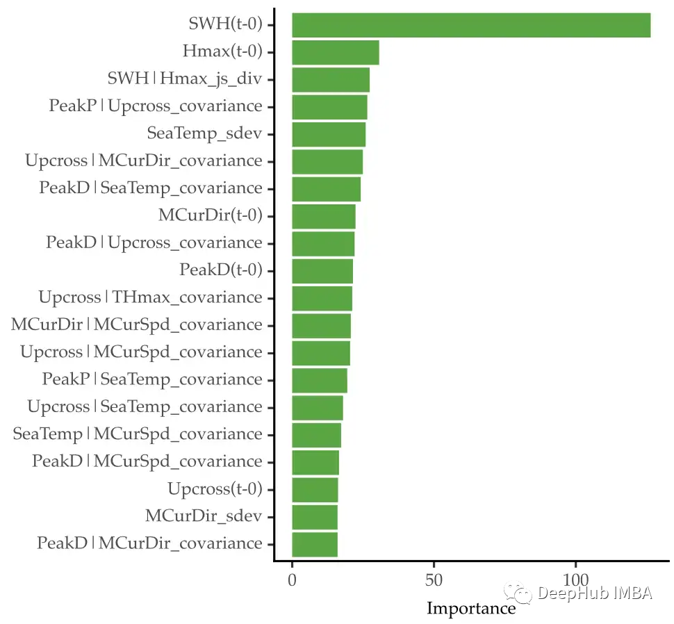
可以看到最重要的特征是目标变量的第一个滞后值。一些提取的特征也出现在前15名中。例如第三个特征SWH|Hmax_js_div。这表示目标变量的滞后与Hmax的滞后之间的Jensen-Shannon散度。第五个特性是SeaTemp_sdev,表示海洋温度的标准偏差滞后。
另一种去除冗余特征的方法是应用相关性过滤器。删除高度相关的特征以减少数据的维数,这里我们就不进行演示了。
总结
本文侧重于多变量时间序列的预测问题。特征提取过程应用于时间序列的多个子序列,在每个时间步骤中,都要用一组统计数据总结过去24小时的数据。
我们也可以用这些统计来一次性描述整个时间序列。如果我们目标是将一组时间序列聚类,那么这可能是很有用。用特征提取总结每个时间序列。然后对得到的特征应用聚类算法。
用几句话总结本文的关键点:
- 多变量时间序列预测通常是一个自回归过程
- 特征工程是数据科学项目中的一个关键步骤。
- 可以用特征工程改进多元时间序列数据。这包括计算单变量和双变量转换和汇总统计信息。
- 提取过多的特征会导致高维问题。可以使用特征选择方法来删除不需要的特征。
本文的数据集在这里下载:
https://erddap.marine.ie/erddap/tabledap/IWaveBNetwork.html.
作者:Vitor Cerqueira