
使用机器学习训练时,如果想训练出精确和健壮的模型需要大量的数据。但当训练模型用于需要自定义数据集的目的时,您通常需要在模型所看到的数据量级上做出妥协。
但是在某些领域就会有一些特殊的情况,例如我们部署到一个地区的任何模型都是使用从前几年的调查中收集的数据建立的,在某些情况下可能是稀疏的(肯定远不及ImageNet[1]等基准数据集的水平)。更糟糕的是,从事某些工作意味着无法使用开放式数据集。
这在某种程度上导致了使用传统机器学习方法部署模型的艰难工作。如果每个类都需要数千个示例,并且随着类的变化,每年都需要重新训练模型,那么为保护构建模型是无用的。但这个问题并不局限于环境保护,基准测试之外的许多领域也存在类似的数据量和变化速率问题。
在本文中,我将讨论一种称为孪生神经网络的模型。希望在阅读之后,您将更好地理解这种体系结构不仅可以帮助保存数据,而且可以帮助数据量有限和类变化速度快的任何领域。
开始
在开始学习之前,你应该对机器学习,特别是卷积神经网络有一定的了解。
您还应该熟悉Python、Keras和TensorFlow。在本文中,我们将介绍一些代码示例。本文中的所有代码都是用TensorFlow 1.14编写的,但是没有理由说这些代码不能在新版本中工作(可能只做了一些修改),或者确实可以移植到其他深度学习框架,比如PyTorch。
什么是孪生神经网络?
简而言之,孪生神经网络是任何包含至少两个并行,相同的卷积神经网络的模型架构。从现在开始,我们将其称为SNN和CNN。这种并行的CNN架构允许模型学习相似性,可以使用相似性代替直接分类。尽管SNN确实在此领域之外使用,但已经发现它们主要用于图像数据,例如面部识别。例如,Selen Uguroglu在NeurIPS 2020上发表了精彩演讲,内容涉及Netflix如何利用SNN来基于电影元数据生成用户推荐。对于本文,我们将重点关注图像数据。
构成SNN一部分的每个并行CNN均设计为产生输入的嵌入或缩小的尺寸表示。例如,如果将嵌入尺寸指定为10,则可以输入尺寸为宽度高度通道的高维图像,并接收直接代表该图像的尺寸为10的浮点值向量作为输出。
这些嵌入可用于优化损失,并在测试时用于生成相似度评分。理论上,平行cnn可以采取任何形式。但重要的一点是,它们必须完全相同;它们必须共享相同的体系结构,共享相同的初始和更新权重,并具有相同的超参数。这种一致性允许模型比较它接收到的输入,通常是每个CNN分支一个。Dey et al.[2]的图章文件提供了一个很好的可视化,如下所示。
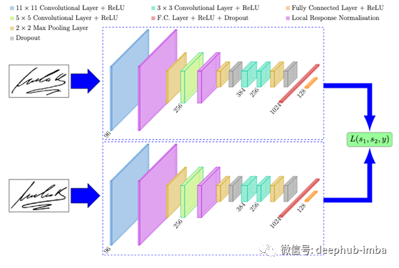
SigNet的目的是确定一个给定的签名是真的还是伪造的。这可以通过使用两个平行的cnn来实现,这些cnn分别对真实和伪造的签名对进行了训练。每个签名通过SNN的一个分支,生成图像的d维嵌入。正是这些嵌入被用来优化损失函数,而不是图像本身。最新版本的snn很可能使用三倍甚至四倍分支,分别包含三个或四个平行的cnn。
SNN的意义是什么?
既然我们理解了SNN的组成,我们就可以强调它们的价值了。使用生成的d维嵌入,我们可以创建一些d维超空间,允许绘制嵌入并创建簇。这个超空间可以用主成分分析(PCA)将其投影到二维进行绘图。
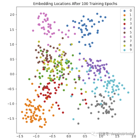
这幅图显示了MNIST测试数据的一个子集[3]的嵌入位置。在这里,一个模型被训练为为10个独特类别(0到9之间的手写数字图像)生成嵌入图像。请注意,即使只经过100次训练,该模型也开始为相同类别的图像生成类似的嵌入图像。这可以通过上图中相同颜色的点的聚类看到——图中的一些聚类是相互叠加的,这是由于PCA将其简化为2d。其他可视化方法,如t-SNE图,或减少到更高的维度,可以在这种情况下提供帮助。
正是这种嵌入簇使snn成为如此强大的工具。如果我们突然决定要向数据中添加另一个类,那么就没有必要对模型进行再训练。新的类嵌入应该以这样一种方式生成,即在绘制到超空间时,它们远离现有的集群,但在添加新类的其他例子时,它们应该与它们聚集在一起。通过使用这种嵌入相似性,我们可以开始用很少的数据为可见和不可见的类产生可能的分类。
模型训练
前面我提到过,snn至少由两个并行的CNN分支组成。SNN中的分支数量对模型训练有很大的影响。您不仅需要确保将数据以每个分支接收训练示例的方式提供给SNN,而且您选择的损失函数还必须考虑分支的数量。无论选择多少支路,损失函数的类型都可能保持一致。
Ranking Losses,也被称为对比损失(Contrastive Losses),旨在预测投影到超空间上的模型输入之间的相对距离。这与预测一组类别标签的更传统的损失相比。Ranking Losses在SNN中起着重要的作用,尽管它们对于其他任务(例如自然语言处理)也很有用。有许多不同类型的Ranking Losses,但是它们(通常)都以相同的方式起作用。
假设我们有两个输入,我们想知道它们有多相似。使用排名损失,我们将执行以下步骤:
- 从输入中提取特征。
- 将提取的特征嵌入到d维超空间中。
- 计算嵌入之间的距离(例如,使用欧几里得距离),以用作相似性的度量。
这里需要注意的是,我们通常并不特别关心嵌入的值,只关心它们之间的距离。以前面显示的嵌入图为例,注意所有点在x轴上约为-1.5,2.0,在y轴上约为-2.0,2.0。嵌入在这个范围内的模型本质上没有好坏之分,重要的是这些点在它们各自的类中聚集。
Triplet Ranking Loss
用于snn的一种更常见的级别损失类型是Triplet Ranking Loss。你经常会看到SNN使用这个叫做三重损失函数,就好像它们是自己的东西一样(事实上,这就是Hoffer等人在最初提出它们的论文[4]中对它们的定义),但实际上它们只是一个SNN,有三个分支。因为三重损失是如此普遍,这是我们将在这篇文章的后面使用的损失函数,了解它是如何工作的很重要。
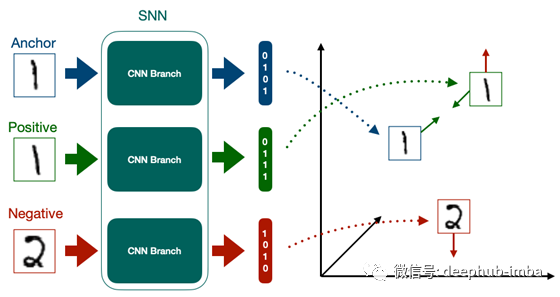
顾名思义,三重损失需要三个输入,我们称之为三元组。三元组中的每个数据点都有其自己的工作。anchor是某个类的数据,它定义了三元组将在哪个类上训练模型。Positive 是类的另一个示例,他的分类与anchor是一样的。Negative 是不是anchor类的另外的类。在训练时,我们的每个三元组组件都被馈送到其自己的CNN分支中进行嵌入。这些嵌入被传递给三重损失函数,该函数定义为:

其中,D(A,P)是 anchor与Positive 之间的嵌入距离,D(A,N)是 anchor与Negative 之间的嵌入距离。我们还定义了一些裕度——它经常使用的初始值是0.2,即FaceNet[5]中使用的裕度。
这个功能的目的是最小化“anchor”与“Positive ”的距离,同时最大化“anchor”与“Positive ”的距离。
Semi-Hard Triplet Mining
我们的SNN必须只提供三个输入,这将使它能够学习。更具体地说,我们希望提供非分类的样本,使我们的模型学习,但这需要花费很长的时间,所以我们需要一个更简单并且省时的方法。
实现这一点的一种简单方法是通过一个称为Semi-Hard Triplet Mining的过程。为了实现这一点,我们首先定义三组三元组:
- Easy Triplets是D(A,P)+边距<D(A,N),因此L = 0的三元组。
- Hard Triplets是D(A,N)<D(A,P)。
- Semi-Hard Triplets是D(A,P)<D(A,N)<D(A,P)+裕度。
目标是找到尽可能多的Semi-Hard Triplet。这些三元组具有正损失,但是正负嵌入距离比负负更接近锚定嵌入。这样可以进行快速训练,但这样对于模型在训练期间实际学习某些东西仍然很困难。
找到这些Semi-Hard Triplet可以用两种方法之一来完成。在离线挖掘中,整个数据集在训练前被转换成三个一集。在在线挖掘中,大量的数据被输入,随机生成三元组。
作为一般经验法则,应该尽可能进行在线挖掘,因为它允许更快的训练,因为它可以随着训练的进展不断更新我们的三元组的阈值定义。这可以通过数据扩充来补充,数据扩充也可以以在线方式执行。
间使用snn进行推理
既然我们了解了snn是如何训练的,接下来我们需要了解如何在推理时使用它们。在训练过程中,我们使用了SNN的所有分支,而推理可以使用单个CNN分支。
在推理时,对未知类的输入图像进行CNN分支处理并嵌入其特征。然后将这种嵌入绘制到超空间上,并与其他簇进行比较。这为我们提供了一个相似性得分的列表,即未知类的图像和所有现有簇之间的相对距离。我们比较输入图像的簇称为支持集。让我们看一个例子来帮助理解这一点。
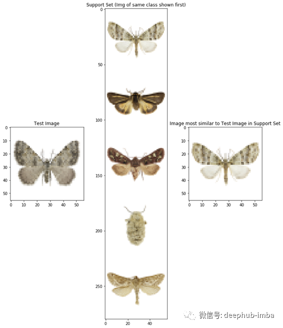
上图是我为确定蛾科而创建的SNN的输出。数据集中的每个图像均改编自Vetrova [6]被标记为五个类的数据。为了便于可视化(尽管事后看来不一定易于理解),每个已知的标记类别都使用来自每个类别的随机示例图像显示在支持集中,如上图中部所示。图的左侧是测试图像。这是SNN看不到的飞蛾图像,SNN现在负责确定分类。
首先,SNN利用训练中学习到的嵌入函数对测试图像进行嵌入。接下来,它将这种嵌入与支持集嵌入进行比较,支持集嵌入为测试图像提供了最可能的蛾类。在图的右边,我们可以看到数据集中的第一个图像被再次打印。
这段代码可以进一步扩展,如果一个嵌入被放置在超空间的新区域,如果嵌入超过了某个预定义的类距离阈值,就会向用户发出警报。这可能表明SNN首次发现了一个新的类别。
我们从哪里测量?
为了确定测试图像和支持集中的类之间的距离,我们需要为每个类提供一个测量的位置。乍一看,似乎可以从每个支持集类中随机选择嵌入,如果所有嵌入都是完全聚集的,那么我们使用哪一个就无关紧要了。
如果我们的类嵌入完美地聚集在一起,这一假设肯定成立,但在现实世界的系统中,情况并非如此。让我们看看下面的示例。
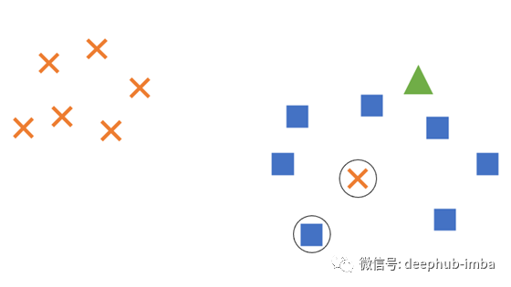
在此示例中,我们有两类嵌入空间,一个用于十字形,一个用于方形。所有方形类别的嵌入都聚集在图的右侧,但是十字架的类别中有一个嵌入尚未与其他嵌入一起聚集在左上角。这个错误的十字形已经被嵌入到方形通常聚集的空间中。右上角还绘制了一个三角形,这是当前的测试图像,已嵌入到空间中,但尚未根据其与其他聚类的距离分配给一个类。
为了确定三角形实际上应该是一个十字形还是一个正方形,我们为每个类别随机选择一个嵌入来进行测量;选择了错误的十字和左下角的正方形(均带圆圈)。如果我们比较这些嵌入的距离,则所选的十字最接近,因此三角形将被标记为十字。
但是,从整体上看,该图很明显应该将三角形标记为正方形,而十字则是一个异常值。通过选择随机嵌入来进行测量,我们就有离群值使距离测量值和最终结果偏斜的风险。
这可以使用原型(prototypes)解决,它是解决我们问题的一种优雅且易于理解的解决方案。原型实质上是每个类别的广义嵌入,从而减少了异常值对距离测量的影响。可以通过多种方法来计算这些值,但是可以采用简单的技术,例如很好地计算中位数。让我们更新示例...
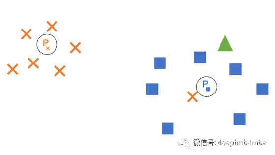
现在,每个类都在其簇的中心附近获得了一个原型(例如Pₓ是交叉类的原型)。如果在测量相似度时选择原型,则三角形将正确标记为正方形。这种简单的解决方案可以大大减少异常值在计算相似度时的影响。
确定应如何计算原型很困难,并且某些数据集可能无法使用诸如中位数之类的解决方案。例如,如果我们所有的交叉类示例在原点周围形成一个半径为1的圆,而正方形类示例在原点周围形成一个半径为2的圆,则原型现在都将在原点处形成,从而实现了相等的距离测量。我们需要找到另一种方法来计算该数据集的原型。
建立孪生神经网络
现在,我们已经掌握了SNN的基本理论,以及为什么它们是重要的工具,下面让我们看一下如何构建SNN。如前所述,我们将为此使用Python,Keras和TensorFlow 1.14,尽管实际上并没有阻止此代码转换为在其他框架(如PyTorch)中使用的代码;我使用TensorFlow是出于个人喜好,而不是因为它更适合制作SNN。为了保持一致性和简化训练,我们还将坚持使用MNIST作为我们的数据集。
这里的代码基于各种资源,我将在本文中进行链接,但是其基础结构是基于Amit Yadav的Coursera中描述的方法,该方法本身就是基于FaceNet [5]。
导入包
首先,我们需要导入所需的程序包。有关在虚拟机上运行此代码所使用的软件包版本的完整列表,请参见此处。我使用Python 3.6.7测试了此代码。
import warnings
warnings.filterwarnings('ignore')

import tensorflow as tf
import matplotlib.pyplot as plt
import numpy as np
import random
import os
import glob

from datetime import datetime
from tensorflow.keras.models import model_from_json
from tensorflow.keras.callbacks import Callback, CSVLogger, ModelCheckpoint
from tensorflow.keras.optimizers import Adam
from tensorflow.keras.layers import Activation, Input, concatenate
from tensorflow.keras.layers import Layer, BatchNormalization, MaxPooling2D, Concatenate, Lambda, Flatten, Dense
from tensorflow.keras.initializers import glorot_uniform, he_uniform
from tensorflow.keras.regularizers import l2
from tensorflow.keras.utils import multi_gpu_model

from sklearn.decomposition import PCA
from sklearn.metrics import roc_curve, roc_auc_score
import math
from pylab import dist
import json

from tensorflow.python.client import device_lib
import matplotlib.gridspec as gridspec
导入资料
接下来,我们需要导入一个数据集以供我们的SNN使用。如前所述,我们将使用MNIST,可以通过TensorFlow的mnist.load_data()进行加载。
加载数据后,将对其进行整形和展平。这样可以更轻松地将数据读取到SNN中。
(x_train, y_train), (x_test, y_test) = tf.keras.datasets.mnist.load_data()

num_classes = len(np.unique(y_train))

x_train_w = x_train.shape[1] # (60000, 28, 28)
x_train_h = x_train.shape[2]
x_test_w = x_test.shape[1]
x_test_h = x_test.shape[2]

x_train_w_h = x_train_w * x_train_h # 28 * 28 = 784
x_test_w_h = x_test_w * x_test_h

x_train = np.reshape(x_train, (x_train.shape[0], x_train_w_h))/255. # (60000, 784)
x_test = np.reshape(x_test, (x_test.shape[0], x_test_w_h))/255.
注意这里我们只有一个高度和宽度,因为MNIST是灰度的,因此只有1个颜色通道。如果我们的数据集具有多个颜色通道,则需要为此修改代码,例如使用x_train_w_h_c。
创建三元组
现在,我们需要创建MNIST三元组。为此需要两种方法。
第一个create_batch()通过随机选择两个类标签(一个用于Anchor / Positive和一个用于Negative)来生成三元组,然后为每个随机选择一个类示例。
def create_batch(batch_size=256, split = "train"):
    x_anchors = np.zeros((batch_size, x_train_w_h))
    x_positives = np.zeros((batch_size, x_train_w_h))
    x_negatives = np.zeros((batch_size, x_train_w_h))

    if split =="train":
        data = x_train
        data_y = y_train
    else:
        data = x_test
        data_y = y_test

    for i in range(0, batch_size):
        # We need to find an anchor, a positive example and a negative example
        random_index = random.randint(0, data.shape[0] - 1)
        x_anchor = data[random_index]
        y = data_y[random_index]

        indices_for_pos = np.squeeze(np.where(data_y == y))
        indices_for_neg = np.squeeze(np.where(data_y != y))

        x_positive = data[indices_for_pos[random.randint(0, len(indices_for_pos) - 1)]]
        x_negative = data[indices_for_neg[random.randint(0, len(indices_for_neg) - 1)]]

        x_anchors[i] = x_anchor
        x_positives[i] = x_positive
        x_negatives[i] = x_negative

    return [x_anchors, x_positives, x_negatives]
第二个create_hard_batch()使用create_batch()创建一批随机三元组,并使用当前的SNN嵌入它们。这使我们能够确定批次中的哪些三元组是Semi-Hard的。如果它们是num_hard,则将其保留为num_hard,并用其他随机三元组填充其余的批处理。通过使用随机三元组进行填充,我们可以开始培训,并确保我们的批次大小一致。
def create_hard_batch(batch_size, num_hard, split = "train"):

    x_anchors = np.zeros((batch_size, x_train_w_h))
    x_positives = np.zeros((batch_size, x_train_w_h))
    x_negatives = np.zeros((batch_size, x_train_w_h))

    if split =="train":
        data = x_train
        data_y = y_train
    else:
        data = x_test
        data_y = y_test

    # Generate num_hard number of hard examples:
    hard_batches = []
    batch_losses = []

    rand_batches = []

    # Get some random batches
    for i in range(0, batch_size):
        hard_batches.append(create_batch(1, split))

        A_emb = embedding_model.predict(hard_batches[i][0])
        P_emb = embedding_model.predict(hard_batches[i][1])
        N_emb = embedding_model.predict(hard_batches[i][2])

        # Compute d(A, P) - d(A, N) for each selected batch
        batch_losses.append(np.sum(np.square(A_emb-P_emb),axis=1) - np.sum(np.square(A_emb-N_emb),axis=1))

    # Sort batch_loss by distance, highest first, and keep num_hard of them
    hard_batch_selections = [x for _, x in sorted(zip(batch_losses,hard_batches), key=lambda x: x[0])]
    hard_batches = hard_batch_selections[:num_hard]

    # Get batch_size - num_hard number of random examples
    num_rand = batch_size - num_hard
    for i in range(0, num_rand):
        rand_batch = create_batch(1, split)
        rand_batches.append(rand_batch)

    selections = hard_batches + rand_batches

    for i in range(0, len(selections)):
        x_anchors[i] = selections[i][0]
        x_positives[i] = selections[i][1]
        x_negatives[i] = selections[i][2]

    return [x_anchors, x_positives, x_negatives]
定义SNN
SNN分为两部分。首先,我们必须创建嵌入模型。该模型接收输入图像并生成d维嵌入。我们在这里创建了一个非常浅的嵌入模型,但是可以创建更复杂的模型。
def create_embedding_model(emb_size):
    embedding_model = tf.keras.models.Sequential([
        Dense(4096,
              activation='relu',
              kernel_regularizer=l2(1e-3),
              kernel_initializer='he_uniform',
              input_shape=(x_train_w_h,)),
        Dense(emb_size,
              activation=None,
              kernel_regularizer=l2(1e-3),
              kernel_initializer='he_uniform')
    ])

    embedding_model.summary()

    return embedding_model
接下来,我们创建一个接收三元组的模型,依次将其传递给嵌入模型进行嵌入,然后将所得嵌入传递给三元组损失函数。
def create_SNN(embedding_model):

    input_anchor = tf.keras.layers.Input(shape=(x_train_w_h,))
    input_positive = tf.keras.layers.Input(shape=(x_train_w_h,))
    input_negative = tf.keras.layers.Input(shape=(x_train_w_h,))

    embedding_anchor = embedding_model(input_anchor)
    embedding_positive = embedding_model(input_positive)
    embedding_negative = embedding_model(input_negative)

    output = tf.keras.layers.concatenate([embedding_anchor, embedding_positive,
                                          embedding_negative], axis=1)

    siamese_net = tf.keras.models.Model([input_anchor, input_positive, input_negative],
                                        output)
    siamese_net.summary()

    return siamese_net
定义三元组损失函数
为了使SNN能够使用三元组进行训练,我们需要定义三元组损失函数。这反映了先前显示的三元组损失函数方程。
def triplet_loss(y_true, y_pred):
    anchor, positive, negative = y_pred[:,:emb_size], y_pred[:,emb_size:2*emb_size],y_pred[:,2*emb_size:]
    positive_dist = tf.reduce_mean(tf.square(anchor - positive), axis=1)
    negative_dist = tf.reduce_mean(tf.square(anchor - negative), axis=1)
    return tf.maximum(positive_dist - negative_dist + alpha, 0.)
定义数据生成器
为了将三元组传递到网络,我们需要创建一个数据生成器功能。TensorFlow在此同时需要x和y,但我们不需要y值,因此我们传递了一个填充符。
def data_generator(batch_size=256, num_hard=50, split="train"):
    while True:
        x = create_hard_batch(batch_size, num_hard, split)
        y = np.zeros((batch_size, 3*emb_size))
        yield x, y
进行训练和评估的设置
现在我们已经定义了SNN的基础,我们可以建立训练模型。首先,我们定义超参数。接下来,我们创建并编译模型。我指定使用CPU执行此操作,但这可能不是必需的,具体取决于您的设置。
编译模型后,我们将存储测试图像嵌入的子集。该模型尚未经过训练,因此这为我们提供了一个很好的基线,以显示在整个训练过程中嵌入如何发生了变化。
# Hyperparams
batch_size = 256
epochs = 100
steps_per_epoch = int(x_train.shape[0]/batch_size)
val_steps = int(x_test.shape[0]/batch_size)
alpha = 0.2
num_hard = int(batch_size * 0.5) # Number of semi-hard triplet examples in the batch
lr = 0.00006
optimiser = 'Adam'
emb_size = 10

with tf.device("/cpu:0"):
    # Create the embedding model
    print("Generating embedding model... \n")
    embedding_model = create_embedding_model(emb_size)

    print("\nGenerating SNN... \n")
    # Create the SNN
    siamese_net = create_SNN(embedding_model)
    # Compile the SNN
    optimiser_obj = Adam(lr = lr)
    siamese_net.compile(loss=triplet_loss, optimizer= optimiser_obj)

    # Store visualisations of the embeddings using PCA for display
    # Create representations of the embedding space via PCA
    embeddings_before_train = loaded_emb_model.predict(x_test[:500, :])
    pca = PCA(n_components=2)
    decomposed_embeddings_before = pca.fit_transform(embeddings_before_train)
现在可以在我们的SNN上进行进一步的评估
def compute_dist(a,b):
return np.linalg.norm(a-b)
def compute_probs(network,X,Y):
'''
Input
network : current NN to compute embeddings
X : tensor of shape (m,w,h,1) containing pics to evaluate
Y : tensor of shape (m,) containing true class
Returns
probs : array of shape (m,m) containing distances
'''
m = X.shape[0]
nbevaluation = int(m*(m-1)/2)
probs = np.zeros((nbevaluation))
y = np.zeros((nbevaluation))
#Compute all embeddings for all imgs with current embedding network
embeddings = embedding_model.predict(X)
k = 0
# For each img in the evaluation set
for i in range(m):
# Against all other images
for j in range(i+1,m):
# compute the probability of being the right decision : it should be 1 for right class, 0 for all other classes
probs[k] = -compute_dist(embeddings[i,:],embeddings[j,:])
if (Y[i]==Y[j]):
y[k] = 1
#print("{3}:{0} vs {1} : \t\t\t{2}\tSAME".format(i,j,probs[k],k, Y[i], Y[j]))
else:
y[k] = 0
#print("{3}:{0} vs {1} : {2}\tDIFF".format(i,j,probs[k],k, Y[i], Y[j]))
k += 1
return probs, y
def compute_metrics(probs,yprobs):
'''
Returns
fpr : Increasing false positive rates such that element i is the false positive rate of predictions with score >= thresholds[i]
tpr : Increasing true positive rates such that element i is the true positive rate of predictions with score >= thresholds[i].
thresholds : Decreasing thresholds on the decision function used to compute fpr and tpr. thresholds[0] represents no instances being predicted and is arbitrarily set to max(y_score) + 1
auc : Area Under the ROC Curve metric
'''
# calculate AUC
auc = roc_auc_score(yprobs, probs)
# calculate roc curve
fpr, tpr, thresholds = roc_curve(yprobs, probs)
return fpr, tpr, thresholds,auc
def draw_roc(fpr, tpr,thresholds, auc):
#find threshold
targetfpr=1e-3
_, idx = find_nearest(fpr,targetfpr)
threshold = thresholds[idx]
recall = tpr[idx]
# plot no skill
plt.plot([0, 1], [0, 1], linestyle='--')
# plot the roc curve for the model
plt.plot(fpr, tpr, marker='.')
plt.title('AUC: {0:.3f}\nSensitivity : {2:.1%} @FPR={1:.0e}\nThreshold={3})'.format(auc,targetfpr,recall,abs(threshold) ))
# show the plot
plt.show()
def find_nearest(array,value):
idx = np.searchsorted(array, value, side="left")
if idx > 0 and (idx == len(array) or math.fabs(value - array[idx-1]) < math.fabs(value - array[idx])):
return array[idx-1],idx-1
else:
return array[idx],idx
def draw_interdist(network, epochs):
interdist = compute_interdist(network)
data = []
for i in range(num_classes):
data.append(np.delete(interdist[i,:],[i]))
fig, ax = plt.subplots()
ax.set_title('Evaluating embeddings distance from each other after {0} epochs'.format(epochs))
ax.set_ylim([0,3])
plt.xlabel('Classes')
plt.ylabel('Distance')
ax.boxplot(data,showfliers=False,showbox=True)
locs, labels = plt.xticks()
plt.xticks(locs,np.arange(num_classes))
plt.show()
def compute_interdist(network):
'''
Computes sum of distances between all classes embeddings on our reference test image:
d(0,1) + d(0,2) + ... + d(0,9) + d(1,2) + d(1,3) + ... d(8,9)
A good model should have a large distance between all theses embeddings
Returns:
array of shape (num_classes,num_classes)
'''
res = np.zeros((num_classes,num_classes))
ref_images = np.zeros((num_classes, x_test_w_h))
#generates embeddings for reference images
for i in range(num_classes):
ref_images[i,:] = x_test[i]
ref_embeddings = network.predict(ref_images)
for i in range(num_classes):
for j in range(num_classes):
res[i,j] = dist(ref_embeddings[i],ref_embeddings[j])
return res
def DrawTestImage(network, images, refidx=0):
'''
Evaluate some pictures vs some samples in the test set
image must be of shape(1,w,h,c)
Returns
scores : result of the similarity scores with the basic images => (N)
'''
nbimages = images.shape[0]
#generates embedings for given images
image_embedings = network.predict(images)
#generates embedings for reference images
ref_images = np.zeros((num_classes,x_test_w_h))
for i in range(num_classes):
images_at_this_index_are_of_class_i = np.squeeze(np.where(y_test == i))
ref_images[i,:] = x_test[images_at_this_index_are_of_class_i[refidx]]
ref_embedings = network.predict(ref_images)
for i in range(nbimages):
# Prepare the figure
fig=plt.figure(figsize=(16,2))
subplot = fig.add_subplot(1,num_classes+1,1)
plt.axis("off")
plotidx = 2
# Draw this image
plt.imshow(np.reshape(images[i], (x_train_w, x_train_h)),vmin=0, vmax=1,cmap='Greys')
subplot.title.set_text("Test image")
for ref in range(num_classes):
#Compute distance between this images and references
dist = compute_dist(image_embedings[i,:],ref_embedings[ref,:])
#Draw
subplot = fig.add_subplot(1,num_classes+1,plotidx)
plt.axis("off")
plt.imshow(np.reshape(ref_images[ref, :], (x_train_w, x_train_h)),vmin=0, vmax=1,cmap='Greys')
subplot.title.set_text(("Class {0}\n{1:.3e}".format(ref,dist)))
plotidx += 1
def evaluate(embedding_model, epochs = 0):
probs,yprob = compute_probs(embedding_model, x_test[:500, :], y_test[:500])
fpr, tpr, thresholds, auc = compute_metrics(probs,yprob)
draw_roc(fpr, tpr, thresholds, auc)
draw_interdist(embedding_model, epochs)
for i in range(3):
DrawTestImage(embedding_model, np.expand_dims(x_train[i],axis=0))
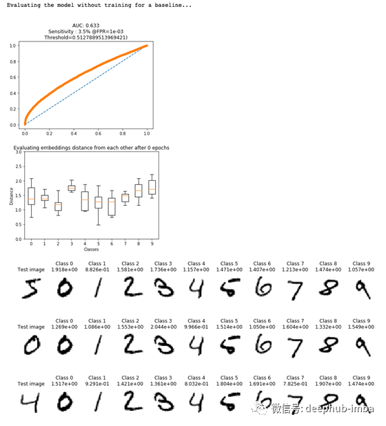
evaluate(embedding_model)
让我们看看对未经训练的模型的评估。从图中可以看出,我们的模型无法区分相似和不相似的图像。这在第三个图中最为明显,它突出显示了测试图像和他们最有可能的类别,而他们的分数之间的差异很小。
现在我们已经编译了模型
def plot_triplets(examples):
    plt.figure(figsize=(6, 2))
    for i in range(3):
        plt.subplot(1, 3, 1 + i)
        plt.imshow(np.reshape(examples[i], (x_train_w, x_train_h)), cmap='binary')
        plt.xticks([])
        plt.yticks([])
    plt.show()

examples = create_batch(1)
print("Example triplet batch:")
plot_triplets(examples)

print("Example semi-hard triplet batch:")
# 1 example, containing 1 semi-hard
ex_hard = create_hard_batch(1, 1, split="train")
plot_triplets(ex_hard)
这会产生以下结果:
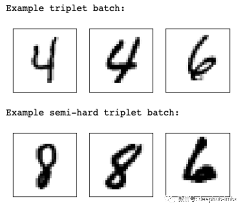
我们的随机三元组示例包含类4的Anchor和Positive,以及类6的Negative。我们的半硬三连音包含第8类的“Anchor”和“Positive”,以及第6类的“Negative”,但请注意它们在组成上是多么相似。
记录模型训练的输出
让我们在训练模型之前设置一些日志记录和自定义回调,以便在以后需要返回时提供帮助。Tensorboard日志回调是改编自erenon的Stack Overflow回答,而基于验证损失保存的最佳模型则是根据OverLordGoldDragon的另一个Stack Overflow答案改编而成。
# Set up logging directory
## Use date-time as logdir name:
#dt = datetime.now().strftime("%Y%m%dT%H%M")
#logdir = os.path.join("PATH/TO/LOG",dt)

## Use a custom non-dt name:
name = "snn-article-example-run"
logdir = os.path.join("PATH/TO/LOG",name)

if not os.path.exists(logdir):
    os.mkdir(logdir)

## Callbacks:
# Create the TensorBoard callback
tensorboard = tf.keras.callbacks.TensorBoard(
    log_dir = logdir,
    histogram_freq=0,
    batch_size=batch_size,
    write_graph=True,
    write_grads=True,
    write_images = True,
    update_freq = 'epoch',
    profile_batch=0
)

# Training logger
csv_log = os.path.join(logdir, 'training.csv')
csv_logger = CSVLogger(csv_log, separator=',', append=True)

# Only save the best model weights based on the val_loss
checkpoint = ModelCheckpoint(os.path.join(logdir, 'snn_model-{epoch:02d}-{val_loss:.2f}.h5'),
                             monitor='val_loss', verbose=1,
                             save_best_only=True, save_weights_only=True,
                             mode='auto')

# Save the embedding mode weights based on the main model's val loss
# This is needed to reecreate the emebedding model should we wish to visualise
# the latent space at the saved epoch
class SaveEmbeddingModelWeights(Callback):
    def __init__(self, filepath, monitor='val_loss', verbose=1):
        super(Callback, self).__init__()
        self.monitor = monitor
        self.verbose = verbose
        self.best = np.Inf
        self.filepath = filepath

    def on_epoch_end(self, epoch, logs={}):
        current = logs.get(self.monitor)
        if current is None:
            warnings.warn("SaveEmbeddingModelWeights requires %s available!" % self.monitor, RuntimeWarning)

        if current < self.best:
            filepath = self.filepath.format(epoch=epoch + 1, **logs)
            if self.verbose == 1:
                print("Saving embedding model weights at %s" % filepath)
            embedding_model.save_weights(filepath, overwrite = True)
            self.best = current

            # Delete the last best emb_model and snn_model
            delete_older_model_files(filepath)

# Save the embedding model weights if you save a new snn best model based on the model checkpoint above
emb_weight_saver = SaveEmbeddingModelWeights(os.path.join(logdir, 'emb_model-{epoch:02d}.h5'))

callbacks = [tensorboard, csv_logger, checkpoint, emb_weight_saver]

# Save model configs to JSON
model_json = siamese_net.to_json()
with open(os.path.join(logdir, "siamese_config.json"), "w") as json_file:
    json_file.write(model_json)
    json_file.close()

model_json = embedding_model.to_json()
with open(os.path.join(logdir, "embedding_config.json"), "w") as json_file:
    json_file.write(model_json)
    json_file.close()

hyperparams = {'batch_size' : batch_size,
              'epochs' : epochs,
               'steps_per_epoch' : steps_per_epoch,
               'val_steps' : val_steps,
               'alpha' : alpha,
               'num_hard' : num_hard,
               'optimiser' : optimiser,
               'lr' : lr,
               'emb_size' : emb_size
              }

with open(os.path.join(logdir, "hyperparams.json"), "w") as json_file:
    json.dump(hyperparams, json_file)

# Set the model to TB
tensorboard.set_model(siamese_net)

def delete_older_model_files(filepath):

    model_dir = filepath.split("emb_model")[0]

    # Get model files
    model_files = os.listdir(model_dir)
    # Get only the emb_model files
    emb_model_files = [file for file in model_files if "emb_model" in file]
    # Get the epoch nums of the emb_model_files
    emb_model_files_epoch_nums = [file.split("-")[1].split(".h5")[0] for file in emb_model_files]

    # Find all the snn model files
    snn_model_files = [file for file in model_files if "snn_model" in file]

    # Sort, get highest epoch num
    emb_model_files_epoch_nums.sort()
    highest_epoch_num = emb_model_files_epoch_nums[-1]

    # Filter the emb_model and snn_model file lists to remove the highest epoch number ones
    emb_model_files_without_highest = [file for file in emb_model_files if highest_epoch_num not in file]
    snn_model_files_without_highest = [file for file in snn_model_files if highest_epoch_num not in file]

    # Delete the non-highest model files from the subdir
    if len(emb_model_files_without_highest) != 0:
        print("Deleting previous best model file:", emb_model_files_without_highest)
        for model_file_list in [emb_model_files_without_highest, snn_model_files_without_highest]:
            for file in model_file_list:
                os.remove(os.path.join(model_dir, file))
训练SNN
现在我们所有的设置已经完成,是时候开始训练了!我首先选择可用gpu的总数,并在这些gpu上并行化模型训练。如果你不能访问多个gpu,你可能需要修改这个。
def get_num_gpus():
    local_device_protos = device_lib.list_local_devices()
    return len([x.name for x in local_device_protos if x.device_type == 'GPU'])

## Training:
print("Logging out to Tensorboard at:", logdir)
print("Starting training process!")
print("-------------------------------------")

# Make the model work over the two GPUs we have
num_gpus = get_num_gpus()
parallel_snn = multi_gpu_model(siamese_net, gpus = num_gpus)
batch_per_gpu = int(batch_size / num_gpus)

parallel_snn.compile(loss=triplet_loss, optimizer= optimiser_obj)

siamese_history = parallel_snn.fit(
    data_generator(batch_per_gpu, num_hard),
    steps_per_epoch=steps_per_epoch,
    epochs=epochs,
    verbose=1,
    callbacks=callbacks,
    workers = 0,
    validation_data = data_generator(batch_per_gpu, num_hard, split="test"),
    validation_steps = val_steps)

print("-------------------------------------")
print("Training complete.")
请注意,在运行model.fit()时,我们提供了训练和测试数据生成器,而不是直接提供训练和测试数据。
评估训练后的模型
一旦模型经过训练,我们就可以评估它并比较它的嵌入。首先,我们加载经过训练的模型。我通过重新加载已保存的日志文件来做到这一点,但如果您只是在一个封闭的系统中运行所有这些,那么一旦模型经过训练,就没有必要重新加载。
一旦模型被加载,我们将执行与未训练模型相同的PCA分解,以可视化嵌入是如何变化的。
def json_to_dict(json_src):
    with open(json_src, 'r') as j:
        return json.loads(j.read())

## Load in best trained SNN and emb model

# The best performing model weights has the higher epoch number due to only saving the best weights
highest_epoch = 0
dir_list = os.listdir(logdir)

for file in dir_list:
    if file.endswith(".h5"):
        epoch_num = int(file.split("-")[1].split(".h5")[0])
        if epoch_num > highest_epoch:
            highest_epoch = epoch_num

# Find the embedding and SNN weights src for the highest_epoch (best) model
for file in dir_list:
    # Zfill ensure a leading 0 on number < 10
    if ("-" + str(highest_epoch).zfill(2)) in file:
        if file.startswith("emb"):
            embedding_weights_src = os.path.join(logdir, file)
        elif file.startswith("snn"):
            snn_weights_src = os.path.join(logdir, file)

hyperparams = os.path.join(logdir, "hyperparams.json")
snn_config = os.path.join(logdir, "siamese_config.json")
emb_config = os.path.join(logdir, "embedding_config.json")

snn_config = json_to_dict(snn_config)
emb_config = json_to_dict(emb_config)

# json.dumps to make the dict a string, as required by model_from_json
loaded_snn_model = model_from_json(json.dumps(snn_config))
loaded_snn_model.load_weights(snn_weights_src)

loaded_emb_model = model_from_json(json.dumps(emb_config))
loaded_emb_model.load_weights(embedding_weights_src)

prototypes = generate_prototypes(x_test, y_test, loaded_emb_model)
# Create representations of the embedding space via PCA
embeddings_after_train = loaded_emb_model.predict(x_test[:500, :])
pca = PCA(n_components=2)
decomposed_embeddings_after = pca.fit_transform(embeddings_after_train)

evaluate(loaded_emb_model)
在上面代码块的末尾,我们再次运行evaluate(),它会生成如下图:
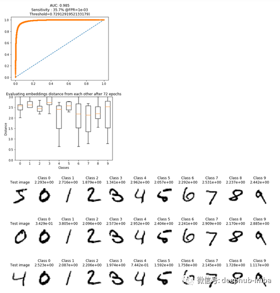
请注意,第一张图现在如何显示AUC为0.985,并且类之间的距离增加了。有趣的是,当查看测试图像及其最可能的类别时,我们可以看到对于第二和第三测试图像,正确地实现了相应的类别(例如,获取类别0的第二测试图像,我们可以看到最低的 所有支持集类别的得分也都在0级,但是从第一个测试图像来看,所有支持集类别的得分都非常接近,这表明训练后的模型在对该图像进行分类时遇到了困难。为了确认我们的模型已经正确训练,并且现在正在形成类簇,让我们绘制先前存储的PCA分解的嵌入图。
step = 1 # Step = 1, take every element

dict_embeddings = {}
dict_gray = {}
test_class_labels = np.unique(np.array(y_test))

decomposed_embeddings_after = pca.fit_transform(embeddings_after_train)

fig = plt.figure(figsize=(16, 8))
for label in test_class_labels:

    y_test_labels = y_test[:num_vis]

    decomposed_embeddings_class_before = decomposed_embeddings_before[y_test_labels == label]
    decomposed_embeddings_class_after = decomposed_embeddings_after[y_test_labels == label]

    plt.subplot(1,2,1)
    plt.scatter(decomposed_embeddings_class_before[::step, 1], decomposed_embeddings_class_before[::step, 0], label=str(label))
    plt.title('Embedding Locations Before Training')
    plt.legend()

    plt.subplot(1,2,2)
    plt.scatter(decomposed_embeddings_class_after[::step, 1], decomposed_embeddings_class_after[::step, 0], label=str(label))
    plt.title('Embedding Locations After %d Training Epochs' % epochs)
    plt.legend()

plt.show()
此代码产生以下输出:
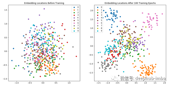
左图显示了训练之前的嵌入位置,使用PCA将其分解为2维以进行可视化,并且每种颜色代表不同的类,如图例所示。请注意,所有嵌入都是如何混杂在一起的,没有清晰的聚类结构,这是有意义的,因为该模型还没有学会将类分离出来。这与右图相反,右图显示了受过训练的SNN嵌入的相同数据点。我们可以在该图的郊区看到清晰的聚类,但是中间仍然显得有些混乱。我们的曲线图表明该模型已经很好地学习了对1类嵌入式图像的聚类(例如,左下角的聚类),但仍与5类嵌入式图像(仍大部分位于中间)较难。这得到了我们以前的图表的支持,该图表显示了该模型正在努力确定最可能匹配5类测试图像的模型。
最好量化模型的性能。这可以使用我们之前讨论的原型,使用n向准确性得分来实现。在n向精度中,将随机选择的测试图像的val_steps个数与大小为n的支持集进行比较。当n与以下代码中的类总数num_class相同时,这提供了模型准确性的指示。MNIST有10类,给出了10类的准确性。
def generate_prototypes(x_data, y_data, embedding_model):
    classes = np.unique(y_data)
    prototypes = {}

    for c in classes:
        #c = classes[0]
        # Find all images of the chosen test class
        locations_of_c = np.where(y_data == c)[0]

        imgs_of_c = x_data[locations_of_c]

        imgs_of_c_embeddings = embedding_model.predict(imgs_of_c)

        # Get the median of the embeddings to generate a prototype for the class (reshaping for PCA)
        prototype_for_c = np.median(imgs_of_c_embeddings, axis = 0).reshape(1, -1)
        # Add it to the prototype dict
        prototypes[c] = prototype_for_c

    return prototypes

 def test_one_shot_prototypes(network, sample_embeddings):
    distances_from_img_to_test_against = []
    # As the img to test against is in index 0, we compare distances between img@0 and all others
    for i in range(1, len(sample_embeddings)):
        distances_from_img_to_test_against.append(compute_dist(sample_embeddings[0], sample_embeddings[i]))
    # As the correct img will be at distances_from_img_to_test_against index 0 (sample_imgs index 1),
    # If the smallest distance in distances_from_img_to_test_against is at index 0,
    # we know the one shot test got the right answer
    is_min = distances_from_img_to_test_against[0] == min(distances_from_img_to_test_against)
    is_max = distances_from_img_to_test_against[0] == max(distances_from_img_to_test_against)
    return int(is_min and not is_max)

def n_way_accuracy_prototypes(n_val, n_way, network):
    num_correct = 0

    for val_step in range(n_val):
        num_correct += load_one_shot_test_batch_prototypes(n_way, network)

    accuracy = num_correct / n_val * 100

    return accuracy

def load_one_shot_test_batch_prototypes(n_way, network):

    labels = np.unique(y_test)
    # Reduce the label set down from size n_classes to n_samples
    labels = np.random.choice(labels, size = n_way, replace = False)

    # Choose a class as the test image
    label = random.choice(labels)
    # Find all images of the chosen test class
    imgs_of_label = np.where(y_test == label)[0]

    # Randomly select a test image of the selected class, return it's index
    img_of_label_idx = random.choice(imgs_of_label)

    # Expand the array at the selected indexes into useable images
    img_of_label = np.expand_dims(x_test[img_of_label_idx],axis=0)

    sample_embeddings = []
    # Get the anchor image embedding
    anchor_prototype = network.predict(img_of_label)
    sample_embeddings.append(anchor_prototype)

    # Get the prototype embedding for the positive class
    positive_prototype = prototypes[label]

    sample_embeddings.append(positive_prototype)

    # Get the negative prototype embeddings
    # Remove the selected test class from the list of labels based on it's index
    label_idx_in_labels = np.where(labels == label)[0]
    other_labels = np.delete(labels, label_idx_in_labels)

    # Get the embedding for each of the remaining negatives
    for other_label in other_labels:
        negative_prototype = prototypes[other_label]
        sample_embeddings.append(negative_prototype)

    correct = test_one_shot_prototypes(network, sample_embeddings)

    return correct

prototypes = generate_prototypes(x_test, y_test, loaded_emb_model)
n_way_accuracy_prototypes(val_steps, num_classes, loaded_emb_model)
当我们运行上述代码时,SNN达到了97.4%的准确率,这是一个值得称赞的分数。由于选择测试图像的随机性,如果愿意,您可以在这里执行交叉验证。
最后,让我们看一下如何生成支持集图像,类似于之前的飞蛾示例所示,只是这次使用MNIST生成。同样,我们将使用10类支持集。
def visualise_n_way_prototypes(n_samples, network):
    labels = np.unique(y_test)
    # Reduce the label set down from size n_classes to n_samples
    labels = np.random.choice(labels, size = n_samples, replace = False)

    # Choose a class as the test image
    label = random.choice(labels)
    # Find all images of the chosen test class
    imgs_of_label = np.where(y_test == label)[0]

    # Randomly select a test image of the selected class, return it's index
    img_of_label_idx = random.choice(imgs_of_label)

    # Get another image idx that we know is of the test class for the sample set
    label_sample_img_idx = random.choice(imgs_of_label)

    # Expand the array at the selected indexes into useable images
    img_of_label = np.expand_dims(x_test[img_of_label_idx],axis=0)
    label_sample_img = np.expand_dims(x_test[label_sample_img_idx],axis=0)

    # Make the first img in the sample set the chosen test image, the second the other image
    sample_imgs = np.empty((0, x_test_w_h))
    sample_imgs = np.append(sample_imgs, img_of_label, axis=0)
    sample_imgs = np.append(sample_imgs, label_sample_img, axis=0)

    sample_embeddings = []

    # Get the anchor embedding image
    anchor_prototype = network.predict(img_of_label)
    sample_embeddings.append(anchor_prototype)

    # Get the prototype embedding for the positive class
    positive_prototype = prototypes[label]
    sample_embeddings.append(positive_prototype)

    # Get the negative prototype embeddings
    # Remove the selected test class from the list of labels based on it's index
    label_idx_in_labels = np.where(labels == label)[0]
    other_labels = np.delete(labels, label_idx_in_labels)
    # Get the embedding for each of the remaining negatives
    for other_label in other_labels:
        negative_prototype = prototypes[other_label]
        sample_embeddings.append(negative_prototype)

        # Find all images of the other class
        imgs_of_other_label = np.where(y_test == other_label)[0]
        # Randomly select an image of the selected class, return it's index
        another_sample_img_idx = random.choice(imgs_of_other_label)
        # Expand the array at the selected index into useable images
        another_sample_img = np.expand_dims(x_test[another_sample_img_idx],axis=0)
        # Add the image to the support set
        sample_imgs = np.append(sample_imgs, another_sample_img, axis=0)

    distances_from_img_to_test_against = []

    # As the img to test against is in index 0, we compare distances between img@0 and all others
    for i in range(1, len(sample_embeddings)):
        distances_from_img_to_test_against.append(compute_dist(sample_embeddings[0], sample_embeddings[i]))

    # + 1 as distances_from_img_to_test_against doesn't include the test image
    min_index = distances_from_img_to_test_against.index(min(distances_from_img_to_test_against)) + 1

    return sample_imgs, min_index

n_samples = 10
sample_imgs, min_index = visualise_n_way_prototypes(n_samples, loaded_emb_model)

img_matrix = []
for index in range(1, len(sample_imgs)):
    img_matrix.append(np.reshape(sample_imgs[index], (x_train_w, x_train_h)))

img_matrix = np.asarray(img_matrix)
img_matrix = np.vstack(img_matrix)

f, ax = plt.subplots(1, 3, figsize = (10, 12))
f.tight_layout()
ax[0].imshow(np.reshape(sample_imgs[0], (x_train_w, x_train_h)),vmin=0, vmax=1,cmap='Greys')
ax[0].set_title("Test Image")
ax[1].imshow(img_matrix ,vmin=0, vmax=1,cmap='Greys')
ax[1].set_title("Support Set (Img of same class shown first)")
ax[2].imshow(np.reshape(sample_imgs[min_index], (x_train_w, x_train_h)),vmin=0, vmax=1,cmap='Greys')
ax[2].set_title("Image most similar to Test Image in Support Set")
这将产生如下图:
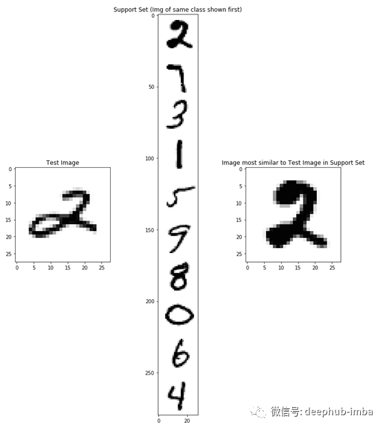
如果本文前面讨论的蛾的例子令人困惑,希望使用MNIST的相同图更清晰。该代码随机选择了第2类测试图像进行分类,并将其与支持集中所有其他类的原型进行比较。同样,绘图代码知道测试图像属于第2类,因此首先显示支持集2。在右边,同样的支持集2再次显示,表明SNN已经正确地为测试图像确定了最可能的2类.
结论
在本文中,我们学习了什么是孪生神经网络,如何训练它们,以及如何在推理时使用它们。即使我们有通过使用MNIST利用例子,我希望它是清楚有力的SNNs可以使用开放式的数据集时,你可能没有所有类可用数据集创建的时候,和如何处理新的训练集未包含类模型。
我希望我已经为你们提供了一个良好的理论知识和实际应用的平衡,我想感谢所有我在文中提到的提供开源代码和Stack Overflow答案的人。没有它,这篇文章以及我自己在保护技术方面的工作就不可能完成。
引用
[1] Deng, J., Dong, W., Socher, R., Li, L.J., Li, K. and Fei-Fei, L., 2009, June. Imagenet: A large-scale hierarchical image database. In 2009 IEEE conference on computer vision and pattern recognition (pp. 248–255). IEEE.
[2] Dey, S., Dutta, A., Toledo, J.I., Ghosh, S.K., Lladós, J. and Pal, U., 2017. Signet: Convolutional siamese network for writer independent offline signature verification. arXiv preprint arXiv:1707.02131.
[3] LeCun, Y., Bottou, L., Bengio, Y. and Haffner, P., 1998. Gradient-based learning applied to document recognition. Proceedings of the IEEE, 86(11), pp.2278–2324.
[4] Hoffer, E. and Ailon, N., 2015, October. Deep metric learning using triplet network. In International Workshop on Similarity-Based Pattern Recognition (pp. 84–92). Springer, Cham.
[5] Schroff, Florian, Dmitry Kalenichenko, and James Philbin. Facenet: A unified embedding for face recognition and clustering. In Proceedings of the IEEE conference on computer vision and pattern recognition, pp. 815–823. 2015.
[6] Vetrova, V., Coup, S., Frank, E. and Cree, M.J., 2018, November. Hidden features: Experiments with feature transfer for fine-grained multi-class and one-class image categorization. In 2018 International Conference on Image and Vision Computing New Zealand (IVCNZ) (pp. 1–6). IEEE.
本文源代码:https://github.com/Trotts/Siamese-Neural-Network-MNIST-Triplet-Loss
作者:Cameron Trotter
原文链接:https://towardsdatascience.com/how-to-train-your-siamese-neural-network-4c6da3259463