
简介
自动驾驶运动规划中会用到各种曲线,主要用于生成车辆的轨迹,常见的轨迹生成算法,如贝塞尔曲线,样条曲线,以及apollo EM Planner的五次多项式曲线,城市场景中使用的是分段多项式曲线,在EM Planner和Lattice Planner中思路是,都是先通过动态规划生成点,再用5次多项式生成曲线连接两个点(虽然后面的版本改动很大,至少lattice planner目前还是这个方法)。
在这里可以看出5次多项式的作用,就是生成轨迹,这里的轨迹不一定是车行驶的轨迹,比如S—T图中的线,是用来做速度规划的。****如下图:
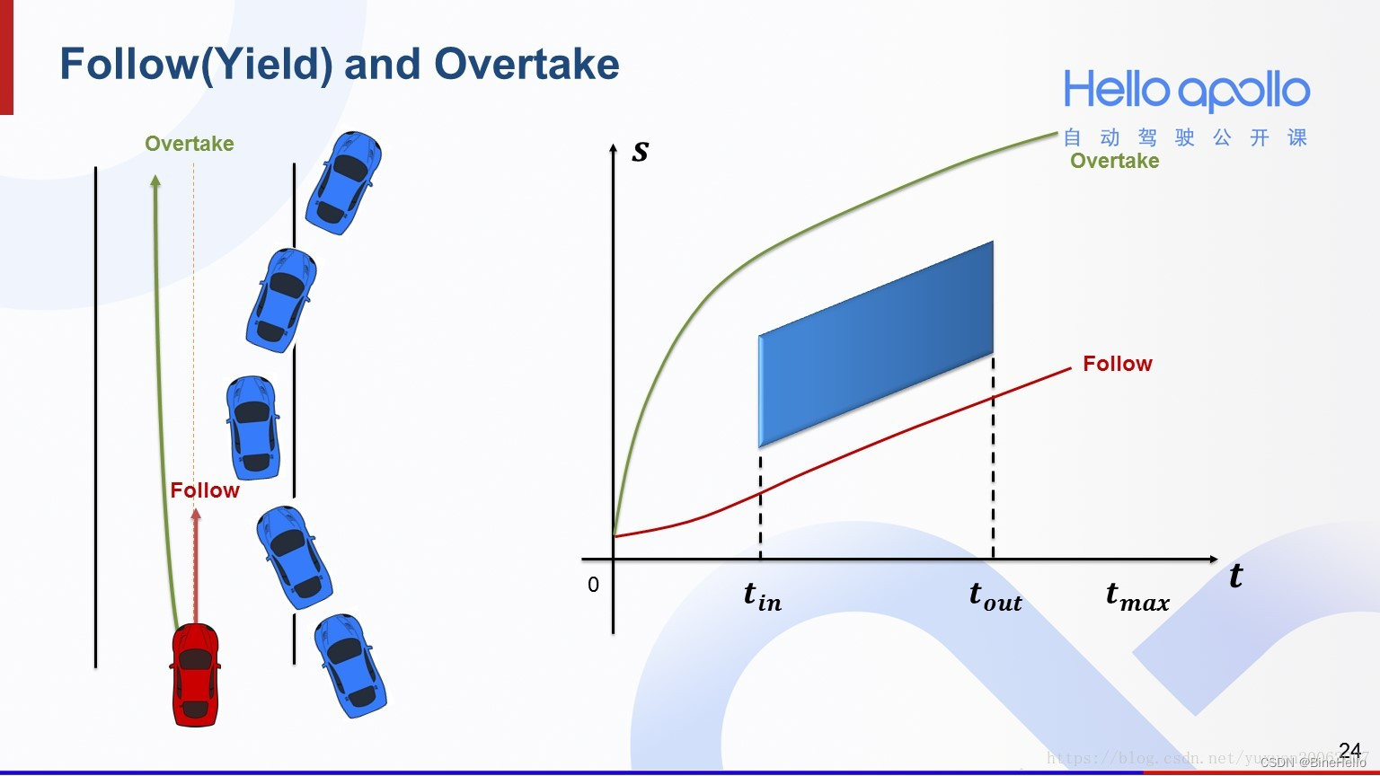
在apollo里面用到了,3-5次多项式,
- cubic_polynomial_curve1d,三次多项式曲线
- quartic_polynomial_curve1d,四次多项式曲线-
- quintic_polynomial_curve1d,五次多项式曲线
3次多项式
f
(
x
)
=
C
0
+
C
1
x
+
C
2
x
2
+
C
3
x
3
−
−
−
−
(
1
)
f(x) = C_0 + C_1x + C_2x^2+ C_3x^3 ----(1)
f(x)=C0+C1x+C2x2+C3x3−−−−(1)
对x求导====>
f
′
(
x
)
=
C
1
+
2
C
2
x
+
3
C
3
x
2
f'(x) = C_1 + 2C_2x+ 3C_3x^2
f′(x)=C1+2C2x+3C3x2
f
(
x
)
=
2
C
2
+
6
C
3
x
f(x) = 2C_2+ 6C_3x
f(x)=2C2+6C3x
因为是连接两个已知点,所以两个轨迹点的信息是已知的。
如已知,当x=0,代如得:
f
(
0
)
=
C
0
;
f
′
(
0
)
=
C
1
;
f
′
′
(
0
)
=
2
C
2
f(0) = C_0 ; f'(0) = C_1;f''(0) =2C_2
f(0)=C0;f′(0)=C1;f′′(0)=2C2
所以
C
0
=
f
(
0
)
;
C
1
=
f
′
(
0
)
;
C
2
=
f
′
′
(
0
)
/
2
C_0 = f(0);C_1 = f'(0); C_2 = f''(0)/2
C0=f(0);C1=f′(0);C2=f′′(0)/2
将终点 (X_end,f(X_end))带入得到C_3。
C
3
=
(
f
(
x
p
)
−
C
0
−
C
1
x
p
−
C
2
x
p
2
)
/
x
p
3
C_3 = (f(x_p)-C_0-C_1x_p-C_2x_p^2)/x_p^3
C3=(f(xp)−C0−C1xp−C2xp2)/xp3
(1)式的所有未知参数都求出,代入x可以得到两点间的轨迹。
apollo中3次多项式的计算
// cubic_polynomial_curve1d.cc
CubicPolynomialCurve1d::CubicPolynomialCurve1d(constdouble x0,constdouble dx0,constdouble ddx0,constdouble x1,constdouble param){ComputeCoefficients(x0, dx0, ddx0, x1, param);
  param_ = param;
  start_condition_[0]= x0;
  start_condition_[1]= dx0;
  start_condition_[2]= ddx0;
  end_condition_ = x1;}void CubicPolynomialCurve1d::ComputeCoefficients(constdouble x0,constdouble dx0,constdouble ddx0,constdouble x1,constdouble param){DCHECK(param >0.0);constdouble p2 = param * param;constdouble p3 = param * p2;
  coef_[0]= x0;
  coef_[1]= dx0;
  coef_[2]=0.5* ddx0;
  coef_[3]=(x1 - x0 - dx0 * param - coef_[2]* p2)/ p3;}
5次多项式
f
(
x
)
=
C
0
+
C
1
x
+
C
2
x
2
+
C
3
x
3
+
C
4
x
4
+
C
5
x
5
−
−
−
−
(
3
−
1
)
f(x) = C_0 + C_1x + C_2x^2+ C_3x^3+C_4x^4+C_5x^5 ----(3-1)
f(x)=C0+C1x+C2x2+C3x3+C4x4+C5x5−−−−(3−1)
对x求导====>
f
′
(
x
)
=
C
1
+
2
C
2
x
+
3
C
3
x
2
+
4
C
4
x
3
+
5
C
5
x
4
−
−
−
−
(
3
−
2
)
f'(x) = C_1 + 2C_2x+ 3C_3x^2+4C_4x^3+5C_5x^4----(3-2)
f′(x)=C1+2C2x+3C3x2+4C4x3+5C5x4−−−−(3−2)
f
′
′
(
x
)
=
2
C
2
+
6
C
3
x
+
12
C
4
x
2
+
20
C
5
x
3
−
−
−
−
(
3
−
3
)
f''(x) = 2C_2+ 6C_3x+12C_4x^2+20C_5x^3----(3-3)
f′′(x)=2C2+6C3x+12C4x2+20C5x3−−−−(3−3)
因为是连接两个已知点,所以两个轨迹点的信息是已知的。
如已知,当x=0,代如得:
f
(
0
)
=
C
0
;
f
′
(
0
)
=
C
1
;
f
′
′
(
0
)
=
2
C
2
f(0) = C_0 ; f'(0) = C_1;f''(0) =2C_2
f(0)=C0;f′(0)=C1;f′′(0)=2C2
所以
C
0
=
f
(
0
)
;
C
1
=
f
′
(
0
)
;
C
2
=
f
′
′
(
0
)
/
2
C_0 = f(0);C_1 = f'(0); C_2 = f''(0)/2
C0=f(0);C1=f′(0);C2=f′′(0)/2
将终点 **(x_e,f(x_e))带入 (3-1) (3-2) (3-3)**。
得到
f
(
x
e
)
=
C
0
+
C
1
x
e
+
C
2
x
e
2
+
C
3
x
e
3
+
C
4
x
e
4
+
C
5
x
e
5
−
−
−
−
(
3
−
4
)
f(x_e) = C_0 + C_1x_e + C_2x_e^2+ C_3x_e^3+C_4x_e^4+C_5x_e^5 ----(3-4)
f(xe)=C0+C1xe+C2xe2+C3xe3+C4xe4+C5xe5−−−−(3−4)
对x求导====>
f
′
(
x
)
=
C
1
+
2
C
2
x
e
+
3
C
3
x
e
2
+
4
C
4
x
e
3
+
5
C
5
x
e
4
−
−
−
−
(
3
−
5
)
f'(x) = C_1 + 2C_2x_e+ 3C_3x_e^2+4C_4x_e^3+5C_5x_e^4----(3-5)
f′(x)=C1+2C2xe+3C3xe2+4C4xe3+5C5xe4−−−−(3−5)
f
′
′
(
x
)
=
2
C
2
+
6
C
3
x
e
+
12
C
4
x
e
2
+
20
C
5
x
e
3
−
−
−
−
(
3
−
6
)
f''(x) = 2C_2+ 6C_3x_e+12C_4x_e^2+20C_5x_e^3----(3-6)
f′′(x)=2C2+6C3xe+12C4xe2+20C5xe3−−−−(3−6)
联立可得
C
3
=
10
(
f
(
x
p
)
−
1
/
2
∗
f
′
′
(
0
)
x
p
2
−
f
′
(
0
)
x
p
−
f
(
0
)
)
−
4
(
f
′
(
x
p
)
−
f
′
′
(
0
)
x
p
−
f
′
(
0
)
)
x
p
+
1
/
2
∗
(
f
′
′
(
x
p
)
−
f
′
′
(
0
)
)
x
p
2
x
p
3
C_3 = \frac{10(f(x_p)-1/2*f''(0)x_p^2-f'(0)x_p-f(0))-4(f'(x_p)-f''(0)x_p-f'(0))x_p+1/2*(f''(x_p)-f''(0))x_p^2}{x_p^3}
C3=xp310(f(xp)−1/2∗f′′(0)xp2−f′(0)xp−f(0))−4(f′(xp)−f′′(0)xp−f′(0))xp+1/2∗(f′′(xp)−f′′(0))xp2
C
4
=
−
15
(
f
(
x
p
)
−
1
/
2
∗
f
′
′
(
0
)
x
p
2
−
f
′
(
0
)
x
p
−
f
(
0
)
)
+
7
(
f
′
(
x
p
)
−
f
′
′
(
0
)
x
p
−
f
′
(
0
)
)
x
p
−
1
/
2
∗
(
f
′
′
(
x
p
)
−
f
′
′
(
0
)
)
x
p
2
x
p
4
C_4 = \frac{-15(f(x_p)-1/2*f''(0)x_p^2-f'(0)x_p-f(0))+7(f'(x_p)-f''(0)x_p-f'(0))x_p-1/2*(f''(x_p)-f''(0))x_p^2}{x_p^4}
C4=xp4−15(f(xp)−1/2∗f′′(0)xp2−f′(0)xp−f(0))+7(f′(xp)−f′′(0)xp−f′(0))xp−1/2∗(f′′(xp)−f′′(0))xp2
C
5
=
6
(
f
(
x
p
)
−
1
/
2
∗
f
′
′
(
0
)
x
p
2
−
f
′
(
0
)
x
p
−
f
(
0
)
)
−
3
(
f
′
(
x
p
)
−
f
′
′
(
0
)
x
p
−
f
′
(
0
)
)
x
p
+
1
/
2
∗
(
f
′
′
(
x
p
)
−
f
′
′
(
0
)
)
x
p
2
x
p
5
C_5 = \frac{6(f(x_p)-1/2*f''(0)x_p^2-f'(0)x_p-f(0))-3(f'(x_p)-f''(0)x_p-f'(0))x_p+1/2*(f''(x_p)-f''(0))x_p^2}{x_p^5}
C5=xp56(f(xp)−1/2∗f′′(0)xp2−f′(0)xp−f(0))−3(f′(xp)−f′′(0)xp−f′(0))xp+1/2∗(f′′(xp)−f′′(0))xp2
apollo中5次多项式的计算
void QuinticPolynomialCurve1d::ComputeCoefficients(constdouble x0,constdouble dx0,constdouble ddx0,constdouble x1,constdouble dx1,constdouble ddx1,constdouble p){CHECK_GT(p,0.0);

  coef_[0]= x0;
  coef_[1]= dx0;
  coef_[2]= ddx0 /2.0;constdouble p2 = p * p;constdouble p3 = p * p2;// the direct analytical method is at least 6 times faster than using matrix// inversion.constdouble c0 =(x1 -0.5* p2 * ddx0 - dx0 * p - x0)/ p3;constdouble c1 =(dx1 - ddx0 * p - dx0)/ p2;constdouble c2 =(ddx1 - ddx0)/ p;

  coef_[3]=0.5*(20.0* c0 -8.0* c1 + c2);
  coef_[4]=(-15.0* c0 +7.0* c1 - c2)/ p;
  coef_[5]=(6.0* c0 -3.0* c1 +0.5* c2)/ p2;}
5次多项式拟合
import math

import matplotlib.pyplot as plt
import numpy as np

# parameter
MAX_T =100.0# maximum time to the goal [s]
MIN_T =5.0# minimum time to the goal[s]

show_animation =TrueclassQuinticPolynomial:def__init__(self, xs, vxs, axs, xe, vxe, axe, time):# calc coefficient of quintic polynomial# See jupyter notebook document for derivation of this equation.# 根据初始状态c0 c1 c2
        self.a0 = xs # x(t)
        self.a1 = vxs # v(t)
        self.a2 = axs /2.0# a(t)

        A = np.array([[time **3, time **4, time **5],[3* time **2,4* time **3,5* time **4],[6* time,12* time **2,20* time **3]])
        b = np.array([xe - self.a0 - self.a1 * time - self.a2 * time **2,
                      vxe - self.a1 -2* self.a2 * time,
                      axe -2* self.a2])# Ax=b 求解x
        x = np.linalg.solve(A, b)# 计算c3 c4 c5
        self.a3 = x[0]
        self.a4 = x[1]
        self.a5 = x[2]# 根据时间计算点x(t)defcalc_point(self, t):
        xt = self.a0 + self.a1 * t + self.a2 * t **2+ \
             self.a3 * t **3+ self.a4 * t **4+ self.a5 * t **5return xt
    # 计算v(t)defcalc_first_derivative(self, t):
        xt = self.a1 +2* self.a2 * t + \
             3* self.a3 * t **2+4* self.a4 * t **3+5* self.a5 * t **4return xt
    # 计算a(t)  defcalc_second_derivative(self, t):
        xt =2* self.a2 +6* self.a3 * t +12* self.a4 * t **2+20* self.a5 * t **3return xt
    # 计算jerk(t)  defcalc_third_derivative(self, t):
        xt =6* self.a3 +24* self.a4 * t +60* self.a5 * t **2return xt

defquintic_polynomials_planner(sx, sy, syaw, sv, sa, gx, gy, gyaw, gv, ga, max_accel, max_jerk, dt):"""
    quintic polynomial planner

    input
        s_x: start x position [m]
        s_y: start y position [m]
        s_yaw: start yaw angle [rad]
        sa: start accel [m/ss]
        gx: goal x position [m]
        gy: goal y position [m]
        gyaw: goal yaw angle [rad]
        ga: goal accel [m/ss]
        max_accel: maximum accel [m/ss]
        max_jerk: maximum jerk [m/sss]
        dt: time tick [s]

    return
        time: time result
        rx: x position result list
        ry: y position result list
        ryaw: yaw angle result list
        rv: velocity result list
        ra: accel result list

    """

    vxs = sv * math.cos(syaw)# 起点速度在x方向分量
    vys = sv * math.sin(syaw)# 起点速度在y方向分量
    vxg = gv * math.cos(gyaw)# 终点速度在x方向分量
    vyg = gv * math.sin(gyaw)# 终点速度在y方向分量

    axs = sa * math.cos(syaw)# 起点加速度在x方向分量
    ays = sa * math.sin(syaw)# 终点加速度在y方向分量
    axg = ga * math.cos(gyaw)# 起点加速度在x方向分量
    ayg = ga * math.sin(gyaw)# 终点加速度在y方向分量

    time, rx, ry, ryaw, rv, ra, rj =[],[],[],[],[],[],[]for T in np.arange(MIN_T, MAX_T, MIN_T):
        xqp = QuinticPolynomial(sx, vxs, axs, gx, vxg, axg, T)
        yqp = QuinticPolynomial(sy, vys, ays, gy, vyg, ayg, T)

        time, rx, ry, ryaw, rv, ra, rj =[],[],[],[],[],[],[]for t in np.arange(0.0, T + dt, dt):
            time.append(t)
            rx.append(xqp.calc_point(t))
            ry.append(yqp.calc_point(t))

            vx = xqp.calc_first_derivative(t)
            vy = yqp.calc_first_derivative(t)
            v = np.hypot(vx, vy)
            yaw = math.atan2(vy, vx)
            rv.append(v)
            ryaw.append(yaw)

            ax = xqp.calc_second_derivative(t)
            ay = yqp.calc_second_derivative(t)
            a = np.hypot(ax, ay)iflen(rv)>=2and rv[-1]- rv[-2]<0.0:
                a *=-1
            ra.append(a)

            jx = xqp.calc_third_derivative(t)
            jy = yqp.calc_third_derivative(t)
            j = np.hypot(jx, jy)iflen(ra)>=2and ra[-1]- ra[-2]<0.0:
                j *=-1
            rj.append(j)ifmax([abs(i)for i in ra])<= max_accel andmax([abs(i)for i in rj])<= max_jerk:print("find path!!")breakif show_animation:# pragma: no coverfor i, _ inenumerate(time):
            plt.cla()# for stopping simulation with the esc key.
            plt.gcf().canvas.mpl_connect('key_release_event',lambda event:[exit(0)if event.key =='escape'elseNone])
            plt.grid(True)
            plt.axis("equal")
            plot_arrow(sx, sy, syaw)
            plot_arrow(gx, gy, gyaw)
            plot_arrow(rx[i], ry[i], ryaw[i])
            plt.title("Time[s]:"+str(time[i])[0:4]+" v[m/s]:"+str(rv[i])[0:4]+" a[m/ss]:"+str(ra[i])[0:4]+" jerk[m/sss]:"+str(rj[i])[0:4],)
            plt.pause(0.001)return time, rx, ry, ryaw, rv, ra, rj

defplot_arrow(x, y, yaw, length=1.0, width=0.5, fc="r", ec="k"):# pragma: no cover"""
    Plot arrow
    """ifnotisinstance(x,float):for(ix, iy, iyaw)inzip(x, y, yaw):
            plot_arrow(ix, iy, iyaw)else:
        plt.arrow(x, y, length * math.cos(yaw), length * math.sin(yaw),
                  fc=fc, ec=ec, head_width=width, head_length=width)
        plt.plot(x, y)defmain():

    sx =10.0# start x position [m]
    sy =10.0# start y position [m]
    syaw = np.deg2rad(10.0)# start yaw angle [rad]
    sv =1.0# start speed [m/s]
    sa =0.1# start accel [m/ss]
    gx =30.0# goal x position [m]
    gy =-10.0# goal y position [m]
    gyaw = np.deg2rad(20.0)# goal yaw angle [rad]
    gv =1.0# goal speed [m/s]
    ga =0.1# goal accel [m/ss]
    max_accel =1.0# max accel [m/ss]
    max_jerk =0.5# max jerk [m/sss]
    dt =0.1# time tick [s]

    time, x, y, yaw, v, a, j = quintic_polynomials_planner(
        sx, sy, syaw, sv, sa, gx, gy, gyaw, gv, ga, max_accel, max_jerk, dt)if show_animation:# pragma: no cover
        plt.plot(x, y,"-r")

        plt.subplots()
        plt.plot(time,[np.rad2deg(i)for i in yaw],"-r")
        plt.xlabel("Time[s]")
        plt.ylabel("Yaw[deg]")
        plt.grid(True)

        plt.subplots()
        plt.plot(time, v,"-r")
        plt.xlabel("Time[s]")
        plt.ylabel("Speed[m/s]")
        plt.grid(True)

        plt.subplots()
        plt.plot(time, a,"-r")
        plt.xlabel("Time[s]")
        plt.ylabel("accel[m/ss]")
        plt.grid(True)

        plt.subplots()
        plt.plot(time, j,"-r")
        plt.xlabel("Time[s]")
        plt.ylabel("jerk[m/sss]")
        plt.grid(True)

        plt.show()if __name__ =='__main__':
    main()
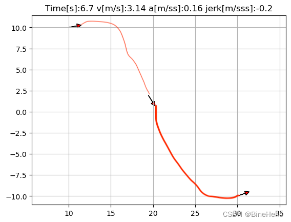
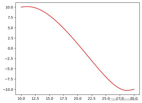
上图模拟了车辆曲线的拟合过程的轨迹,箭头代表方向。
过程的速度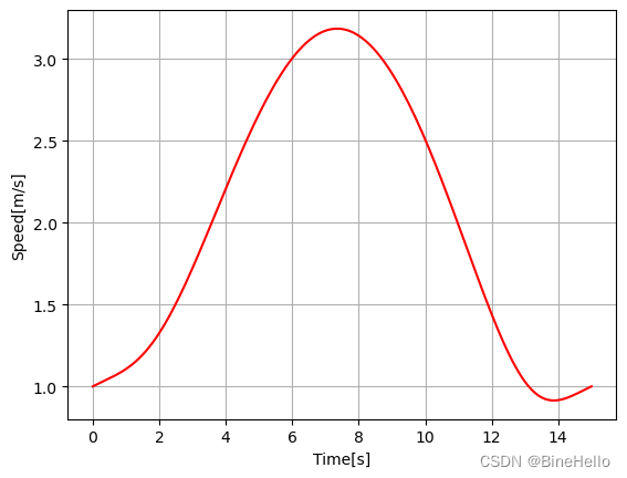
感觉5次多项式和贝塞尔曲线还是挺像的,有时间写一篇五次多项式、贝塞尔曲线、样条曲线的对比。
还有一个问题就是为啥要用5次多项式,而不是4次,6次更高阶或者低阶呢?下回复习一下老王的讲解。
参考:
本文转载自: https://blog.csdn.net/weixin_43673156/article/details/129016974
版权归原作者 BineHello 所有, 如有侵权,请联系我们删除。
版权归原作者 BineHello 所有, 如有侵权,请联系我们删除。