换个新头像（解决彩色图亮度不均衡）

文章目录

前言

CSDN博客好久没有换过头像了，想换个新头像，在相册里面翻来翻去，然后就找到以前养的小宠物的一些照片，有一张特别有意思
在这里插入图片描述
惊恐到站起来的金丝熊：这家伙不会要吃我吧

没见过仓鼠的小猫：这啥玩意儿？

好，就决定把这张图当自己的头像了

一顿操作之后，把头像换成了这张照片

在这里插入图片描述

此时我：啥玩意儿？

。。。。感觉黑乎乎的，啥也看不清
这时候我想起来我学过图像处理，这用亮度变换搞一下不就可以了吗，搞起来！

注意：一般对灰度图进行亮度变换的多一点，但是我这张图是RGB图（准确来说是RGBA，但我们只取前三个通道），对于RGB图，我这里对其每个通道分别进行处理然后拼接处理

处理

对比度拉伸

也就是把图像重新缩放到指定的范围内

# 对比度拉伸
p1, p2 = np.percentile(img,(0,70))# numpy计算多维数组的任意百分比分位数
rescale_img = np.uint8((np.clip(img, p1, p2)- p1)/(p2 - p1)*255)

其中，numpy的percentile函数可以计算多维数组的任意百分比分位数，因为我的图片中整体偏暗，我就把原图灰度值的0% ~ 70%缩放到0 ~255

log变换

使用以下公式进行映射：

     O
    
    
     =
    
    
     g
    
    
     a
    
    
     i
    
    
     n
    
    
     ∗
    
    
     l
    
    
     o
    
    
     g
    
    
     (
    
    
     1
    
    
     +
    
    
     I
    
    
     )
    
   
   
    O = gain*log(1 + I)
   
  
 O=gain∗log(1+I)

# 对数变换
log_img = np.zeros_like(img)
scale, gain =255,1.5for i inrange(3):
    log_img[:,:, i]= np.log(img[:,:, i]/ scale +1)* scale * gain

Gamma校正

使用以下公式进行映射：

     O
    
    
     =
    
    
     
      I
     
     
      γ
     
    
    
     ∗
    
    
     g
    
    
     a
    
    
     i
    
    
     n
    
   
   
    O = I^{\gamma} * gain
   
  
 O=Iγ∗gain

# gamma变换
gamma, gain, scale =0.7,1,255
gamma_img = np.zeros_like(img)for i inrange(3):
    gamma_img[:,:, i]=((img[:,:, i]/ scale)** gamma)* scale * gain

直方图均衡化

使用直方图均衡后的图像具有大致线性的累积分布函数，其优点是不需要参数。
其原理为，考虑这样一个图像，它的像素值被限制在某个特定的值范围内，即灰度范围不均匀。所以我们需要将其直方图缩放遍布整个灰度范围(如下图所示，来自维基百科)，这就是直方图均衡化所做的(简单来说)。这通常会提高图像的对比度。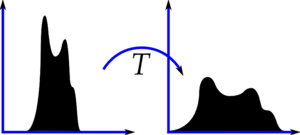
在这里插入图片描述

这里使用OpenCV来演示。

# 直方图均衡化
equa_img = np.zeros_like(img)for i inrange(3):
    equa_img[:,:, i]= cv.equalizeHist(img[:,:, i])

对比度自适应直方图均衡化(CLAHE)

这是一种自适应直方图均衡化方法
OpenCV提供了该方法。

# 对比度自适应直方图均衡化
clahe_img = np.zeros_like(img)
clahe = cv.createCLAHE(clipLimit=2.0, tileGridSize=(8,8))for i inrange(3):
    clahe_img[:,:, i]= clahe.apply(img[:,:, i])

处理结果展示

使用Matplotlib显示上述几种方法的结果：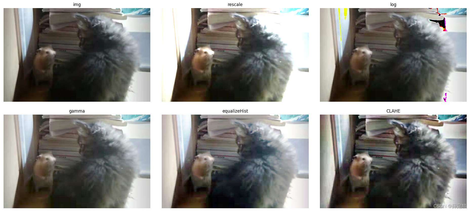
在这里插入图片描述
可以看到，前四种方法效果都差不多，都有一个问题亮的地方过于亮，这是因为他们考虑的是全局对比度，而且因为我们使用的彩色图像原因，使用log变换的结果图中有部分区域色彩失真。最后一种CLAHE方法考虑的是局部对比度，所以效果会好一点。

因为图像是彩色的，这里我只绘制了R通道的直方图（红色线）及其累积分布函数（黑色线）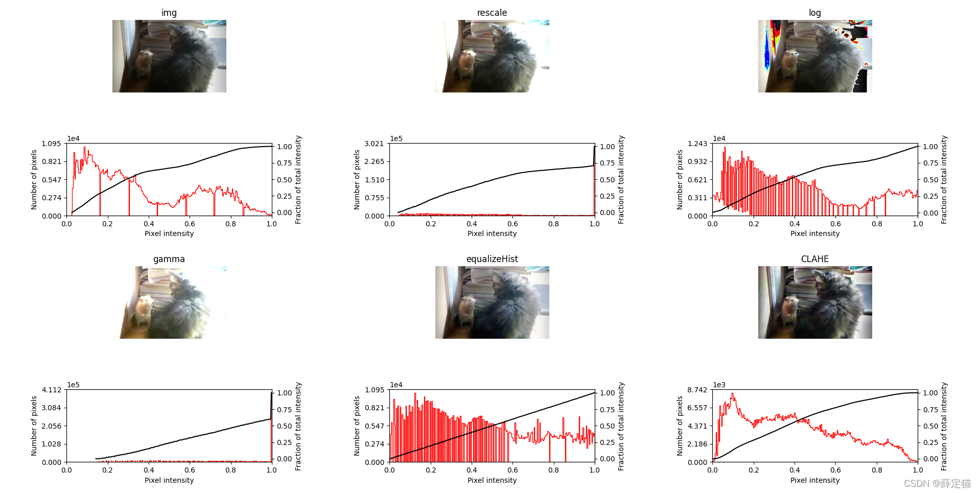
在这里插入图片描述

可以看到均衡后的图像具有大致线性的累积分布函数。

总之，经过以上的探索，我最终决定使用CLAHE均衡后的结果

在这里插入图片描述
感觉是比之前的好了点

附源码

opencv版本

import cv2.cv2 as cv
import matplotlib.pyplot as plt
import numpy as np

defplot_img_and_hist(image, axes, bins=256):"""Plot an image along with its histogram and cumulative histogram.

    """
    ax_img, ax_hist = axes
    ax_cdf = ax_hist.twinx()# Display image
    ax_img.imshow(image, cmap=plt.cm.gray)
    ax_img.set_axis_off()# Display histogram
    colors =['red','green','blue']for i inrange(1):
        ax_hist.hist(image[:,:, i].ravel(), bins=bins, histtype='step', color=colors[i])

    ax_hist.ticklabel_format(axis='y', style='scientific', scilimits=(0,0))

    ax_hist.set_xlabel('Pixel intensity')
    ax_hist.set_xlim(0,255)# 这里范围为0~255 如果使用img_as_float，则这里为0~1
    ax_hist.set_yticks([])# Display cumulative distributionfor i inrange(1):
        hist, bins = np.histogram(image[:,:, i].flatten(),256,[0,256])
        cdf = hist.cumsum()
        cdf = cdf *float(hist.max())/ cdf.max()
        ax_cdf.plot(bins[1:], cdf,'k')
    ax_cdf.set_yticks([])return ax_img, ax_hist, ax_cdf

defplot_all(images, titles, cols):"""
    输入titles、images、以及每一行多少列，自动计算行数、并绘制图像和其直方图
    :param images:
    :param titles:
    :param cols: 每一行多少列
    :return:
    """
    fig = plt.figure(figsize=(12,8))
    img_num =len(images)# 图片的个数
    rows =int(np.ceil(img_num / cols)*2)# 上图下直方图 所以一共显示img_num*2个子图
    axes = np.zeros((rows, cols), dtype=object)
    axes = axes.ravel()
    axes[0]= fig.add_subplot(rows, cols,1)# 先定义第一个img 单独拿出来定义它是为了下面的sharex# 开始创建所有的子窗口for i inrange(1, img_num):#
        axes[i + i // cols * cols]= fig.add_subplot(rows, cols, i + i // cols * cols +1, sharex=axes[0],
                                                     sharey=axes[0])for i inrange(0, img_num):
        axes[i + i // cols * cols + cols]= fig.add_subplot(rows, cols, i + i // cols * cols + cols +1)for i inrange(0, img_num):# 这里从1开始，因为第一个在上面已经绘制过了
        ax_img, ax_hist, ax_cdf = plot_img_and_hist(images[i],(axes[i + i // cols * cols], axes[i + i // cols * cols + cols]))
        ax_img.set_title(titles[i])
        y_min, y_max = ax_hist.get_ylim()
        ax_hist.set_ylabel('Number of pixels')
        ax_hist.set_yticks(np.linspace(0, y_max,5))

        ax_cdf.set_ylabel('Fraction of total intensity')
        ax_cdf.set_yticks(np.linspace(0,1,5))# prevent overlap of y-axis labels
    fig.tight_layout()
    plt.show()
    plt.close(fig)if __name__ =='__main__':
    img = cv.imread('catandmouse.png', cv.IMREAD_UNCHANGED)[:,:,:3]
    img = cv.cvtColor(img, cv.COLOR_BGR2RGB)

    gray = cv.cvtColor(img, cv.COLOR_BGR2GRAY)# 对比度拉伸
    p1, p2 = np.percentile(img,(0,70))# numpy计算多维数组的任意百分比分位数
    rescale_img = np.uint8((np.clip(img, p1, p2)- p1)/(p2 - p1)*255)# 对数变换
    log_img = np.zeros_like(img)
    scale, gain =255,1.5for i inrange(3):
        log_img[:,:, i]= np.log(img[:,:, i]/ scale +1)* scale * gain

    # gamma变换
    gamma, gain, scale =0.7,1,255
    gamma_img = np.zeros_like(img)for i inrange(3):
        gamma_img[:,:, i]=((img[:,:, i]/ scale)** gamma)* scale * gain

    # 彩色图直方图均衡化# 直方图均衡化
    equa_img = np.zeros_like(img)for i inrange(3):
        equa_img[:,:, i]= cv.equalizeHist(img[:,:, i])# 对比度自适应直方图均衡化
    clahe_img = np.zeros_like(img)
    clahe = cv.createCLAHE(clipLimit=2.0, tileGridSize=(8,8))for i inrange(3):
        clahe_img[:,:, i]= clahe.apply(img[:,:, i])

    titles =['img','rescale','log','gamma','equalizeHist','CLAHE']
    images =[img, rescale_img, log_img, gamma_img, equa_img, clahe_img]
    plot_all(images, titles,3)

skimage版本

from skimage import exposure, util, io, color, filters, morphology
import matplotlib.pyplot as plt
import numpy as np

defplot_img_and_hist(image, axes, bins=256):"""Plot an image along with its histogram and cumulative histogram.

    """
    image = util.img_as_float(image)
    ax_img, ax_hist = axes
    ax_cdf = ax_hist.twinx()# Display image
    ax_img.imshow(image, cmap=plt.cm.gray)
    ax_img.set_axis_off()# Display histogram
    colors =['red','green','blue']for i inrange(1):
        ax_hist.hist(image[:,:, i].ravel(), bins=bins, histtype='step', color=colors[i])

    ax_hist.ticklabel_format(axis='y', style='scientific', scilimits=(0,0))
    ax_hist.set_xlabel('Pixel intensity')
    ax_hist.set_xlim(0,1)
    ax_hist.set_yticks([])# Display cumulative distributionfor i inrange(1):
        img_cdf, bins = exposure.cumulative_distribution(image[:,:, i], bins)
        ax_cdf.plot(bins, img_cdf,'k')
    ax_cdf.set_yticks([])return ax_img, ax_hist, ax_cdf

defplot_all(images, titles, cols):"""
    输入titles、images、以及每一行多少列，自动计算行数、并绘制图像和其直方图
    :param images:
    :param titles:
    :param cols: 每一行多少列
    :return:
    """
    fig = plt.figure(figsize=(12,8))
    img_num =len(images)# 图片的个数
    rows =int(np.ceil(img_num / cols)*2)# 上图下直方图 所以一共显示img_num*2个子图
    axes = np.zeros((rows, cols), dtype=object)
    axes = axes.ravel()
    axes[0]= fig.add_subplot(rows, cols,1)# 先定义第一个img 单独拿出来定义它是为了下面的sharex# 开始创建所有的子窗口for i inrange(1, img_num):#
        axes[i + i // cols * cols]= fig.add_subplot(rows, cols, i + i // cols * cols +1, sharex=axes[0],
                                                     sharey=axes[0])for i inrange(0, img_num):
        axes[i + i // cols * cols + cols]= fig.add_subplot(rows, cols, i + i // cols * cols + cols +1)for i inrange(0, img_num):# 这里从1开始，因为第一个在上面已经绘制过了
        ax_img, ax_hist, ax_cdf = plot_img_and_hist(images[i],(axes[i + i // cols * cols], axes[i + i // cols * cols + cols]))
        ax_img.set_title(titles[i])
        y_min, y_max = ax_hist.get_ylim()
        ax_hist.set_ylabel('Number of pixels')
        ax_hist.set_yticks(np.linspace(0, y_max,5))

        ax_cdf.set_ylabel('Fraction of total intensity')
        ax_cdf.set_yticks(np.linspace(0,1,5))# prevent overlap of y-axis labels
    fig.tight_layout()
    plt.show()
    plt.close(fig)if __name__ =='__main__':
    img = io.imread('catandmouse.png')[:,:,:3]

    gray = color.rgb2gray(img)# 对比度拉伸
    p1, p2 = np.percentile(img,(0,70))# numpy计算多维数组的任意百分比分位数
    rescale_img = exposure.rescale_intensity(img, in_range=(p1, p2))# 对数变换# img = util.img_as_float(img)
    log_img = np.zeros_like(img)for i inrange(3):
        log_img[:,:, i]= exposure.adjust_log(img[:,:, i],1.2,False)# gamma变换
    gamma_img = np.zeros_like(img)for i inrange(3):
        gamma_img[:,:, i]= exposure.adjust_gamma(img[:,:, i],0.7,2)# 彩色图直方图均衡化
    equa_img = np.zeros_like(img, dtype=np.float64)# 注意直方图均衡化输出值为float类型的for i inrange(3):
        equa_img[:,:, i]= exposure.equalize_hist(img[:,:, i])# 对比度自适应直方图均衡化
    clahe_img = np.zeros_like(img, dtype=np.float64)for i inrange(3):
        clahe_img[:,:, i]= exposure.equalize_adapthist(img[:,:, i])# 局部直方图均衡化 效果不好就不放了
    selem = morphology.rectangle(50,50)
    loc_img = np.zeros_like(img)for i inrange(3):
        loc_img[:,:, i]= filters.rank.equalize(util.img_as_ubyte(img[:,:, i]), footprint=selem)# Display results
    titles =['img','rescale','log','gamma','equalizeHist','CLAHE']
    images =[img, rescale_img, log_img, gamma_img, equa_img, clahe_img]

    plot_all(images, titles,3)

标签： python 机器学习计算机视觉

本文转载自: https://blog.csdn.net/weixin_44456692/article/details/122235564
版权归原作者 薛定猫 所有，如有侵权，请联系我们删除。

换个新头像（解决彩色图亮度不均衡）

文章目录

前言

处理

对比度拉伸

log变换

Gamma校正

直方图均衡化

对比度自适应直方图均衡化(CLAHE)

处理结果展示

附源码

opencv版本

skimage版本

发表评论

“换个新头像（解决彩色图亮度不均衡）”的评论:

关于作者

overfit同步小助手

相关阅读

文章导航