
高斯混合模型(后面本文中将使用他的缩写 GMM)听起来很复杂,其实他的工作原理和 KMeans 非常相似,你甚至可以认为它是 KMeans 的概率版本。 这种概率特征使 GMM 可以应用于 KMeans 无法解决的许多复杂问题。
因为KMeans的限制很多,比如: 它假设簇是球形的并且大小相同,这在大多数现实世界的场景中是无效的。并且它是硬聚类方法,这意味着每个数据点都分配给一个集群,这也是不现实的。
在本文中,我们将根据上面的内容来介绍 KMeans 的一个替代方案之一,高斯混合模型。
从概念上解释:高斯混合模型就是用高斯概率密度函数(正态分布曲线)精确地量化事物,它是一个将事物分解为若干的基于高斯概率密度函数(正态分布曲线)形成的模型。
高斯混合模型 (GMM) 算法的工作原理
正如前面提到的,可以将 GMM 称为 概率的KMeans,这是因为 KMeans 和 GMM 的起点和训练过程是相同的。 但是,KMeans 使用基于距离的方法,而 GMM 使用概率方法。 GMM 中有一个主要假设:数据集由多个高斯分布组成,换句话说,GMM 模型可以看作是由 K 个单高斯模型组合而成的模型,这 K 个子模型是混合模型的隐变量(Hidden variable)
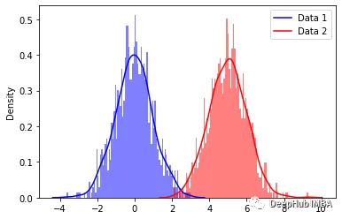
上述分布通常称为多模型分布。 每个峰代表我们数据集中不同的高斯分布或聚类。 我们肉眼可以看到这些分布,但是使用公式如何估计这些分布呢?
在解释这个问题之前,我们先创建一些高斯分布。这里我们生成的是多元正态分布; 它是单变量正态分布的更高维扩展。
让我们定义数据点的均值和协方差。 使用均值和协方差,我们可以生成如下分布。
 # Set the mean and covariance
 mean1= [0, 0]
 mean2= [2, 0]
 cov1= [[1, .7], [.7, 1]]
 cov2= [[.5, .4], [.4, .5]]

 # Generate data from the mean and covariance
 data1=np.random.multivariate_normal(mean1, cov1, size=1000)
 data2=np.random.multivariate_normal(mean2, cov2, size=1000)
可视化一下生成的数据
 plt.figure(figsize=(10,6))

 plt.scatter(data1[:,0],data1[:,1])
 plt.scatter(data2[:,0],data2[:,1])

 sns.kdeplot(data1[:, 0], data1[:, 1], levels=20, linewidth=10, color='k', alpha=0.2)
 sns.kdeplot(data2[:, 0], data2[:, 1], levels=20, linewidth=10, color='k', alpha=0.2)

 plt.grid(False)
 plt.show()
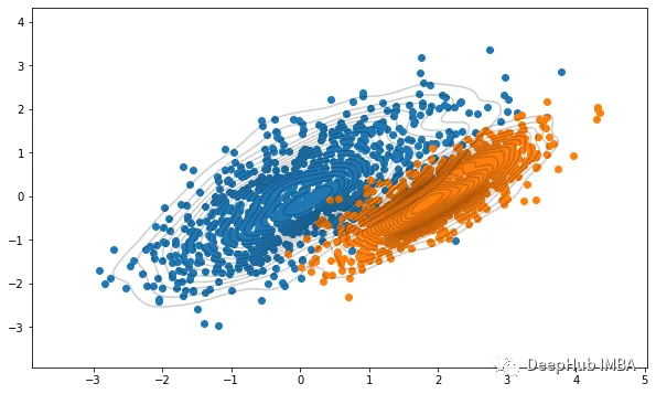
我们上面所做的工作是:使用均值和协方差矩阵生成了随机高斯分布。 而 GMM 要做正好与这个相反,也就是找到一个分布的均值和协方差,那么怎么做呢?
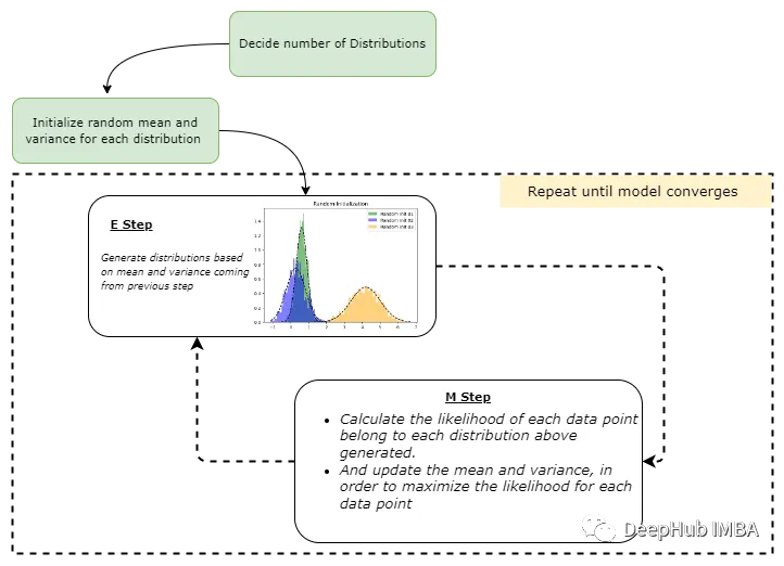
工作过程大致如下:
为给定的数据集确定聚类的数量(这里我们可以使用领域知识或其他方法,例如 BIC/AIC)。 根据我们上面的参数,有 1000 个数据点,和两个簇2。
初始化每个簇的均值、协方差和权重参数。
使用期望最大化算法执行以下操作:
- 期望步骤(E-step):计算每个数据点属于每个分布的概率,然后使用参数的当前估计评估似然函数
- 最大化步骤(M-step):更新之前的均值、协方差和权重参数,这样最大化E步骤中找到的预期似然
- 重复这些步骤,直到模型收敛。
以上是GMM 算法的非数学的通俗化的解释。
GMM 数学原理
有了上面的通俗解释,我们开始进入正题,上面的解释可以看到GMM 的核心在于上一节中描述的期望最大化 (EM) 算法。
在解释之前,我们先演示一下 EM 算法在 GMM 中的应用。
1、初始化均值、协方差和权重参数
- mean (μ): 随机初始化
- 协方差 (Σ):随机初始化
- 权重(混合系数)(π):每个类的分数是指特定数据点属于每个类的可能性。 一开始,这对所有簇都是平等的。 假设我们用三个分量拟合 GMM,那么每个组件的权重参数可能设置为 1/3,这样概率分布为 (1/3, 1/3, 1/3)。
2、期望步骤(E-step)
对于每个数据点𝑥𝑖,使用以下等式计算数据点属于簇 (𝑐) 的概率。 这里的k是我分布(簇)数。

上面的𝜋_𝑐是高斯分布c的混合系数(有时称为权重),它在上一阶段被初始化,𝑁(𝒙|𝝁,𝚺)描述了高斯分布的概率密度函数(PDF),均值为𝜇和 关于数据点 x 的协方差 Σ; 所以可以有如下表示。

E-step 使用模型参数的当前估计值计算概率。 这些概率通常称为高斯分布的“responsibilities”。 它们由变量 r_ic 表示,其中 i 是数据点的索引,c 是高斯分布的索引。 responsibilities衡量第 c 个高斯分布对生成第 i 个数据点“负责”的程度。 这里使用条件概率,更具体地说是贝叶斯定理。
一个简单的例子。 假设我们有 100 个数据点,需要将它们聚类成两组。 我们可以这样写 r_ic(i=20,c=1) 。 其中 i 代表数据点的索引,c 代表我们正在考虑的簇的索引。
不要忘记在开始时,𝜋_𝑐 会初始化为等值。 在我们的例子中,𝜋_1 = 𝜋_2 = 1/2。

E-step 的结果是混合模型中每个数据点和每个高斯分布的一组responsibilities。 这些responsibilities会在 M-step更新模型参数的估计。
3、最大化步骤(M-step)
算法使用高斯分布的responsibilities(在 E-step中计算的)来更新模型参数的估计值。
M-step更新参数的估计如下:

上面的公式 4 更新 πc(混合系数),公式 5 更新 μc,公式6 更新 Σc。更新后的的估计会在下一个 E-step 中用于计算数据点的新responsibilities。
GMM 将将重复这个过程直到算法收敛,通常在模型参数从一次迭代到下一次迭代没有显着变化时就被认为收敛了。
让我们将上面的过程整理成一个简单的流程图,这样可以更好的理解:
数学原理完了,下面该开始使用 Python 从头开始实现 GMM了
使用 Python 从头开始实现 GMM
理解了数学原理,GMM的代码也不复杂,基本上上面的每一个公式使用1-2行就可以完成
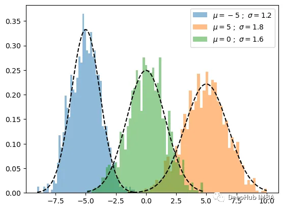
首先,创建一个实验数据集,我们将为一维数据集实现 GMM,因为这个比较简单
 importnumpyasnp

 n_samples=100
 mu1, sigma1=-5, 1.2
 mu2, sigma2=5, 1.8
 mu3, sigma3=0, 1.6

 x1=np.random.normal(loc=mu1, scale=np.sqrt(sigma1), size=n_samples)
 x2=np.random.normal(loc=mu2, scale=np.sqrt(sigma2), size=n_samples)
 x3=np.random.normal(loc=mu3, scale=np.sqrt(sigma3), size=n_samples)

 X=np.concatenate((x1,x2,x3))
下面是可视化的函数封装
 fromscipy.statsimportnorm

 defplot_pdf(mu,sigma,label,alpha=0.5,linestyle='k--',density=True):
     """
     Plot 1-D data and its PDF curve.

     """
     # Compute the mean and standard deviation of the data

     # Plot the data

     X=norm.rvs(mu, sigma, size=1000)

     plt.hist(X, bins=50, density=density, alpha=alpha,label=label)

     # Plot the PDF
     x=np.linspace(X.min(), X.max(), 1000)
     y=norm.pdf(x, mu, sigma)
     plt.plot(x, y, linestyle)
并绘制生成的数据如下。 这里没有绘制数据本身,而是绘制了每个样本的概率密度。
 plot_pdf(mu1,sigma1,label=r"$\mu={} \ ; \ \sigma={}$".format(mu1,sigma1))
 plot_pdf(mu2,sigma2,label=r"$\mu={} \ ; \ \sigma={}$".format(mu2,sigma2))
 plot_pdf(mu3,sigma3,label=r"$\mu={} \ ; \ \sigma={}$".format(mu3,sigma3))
 plt.legend()
 plt.show()
下面开始根据上面的公式实现代码:
1、初始化
 defrandom_init(n_compenents):

     """Initialize means, weights and variance randomly
       and plot the initialization
     """

     pi=np.ones((n_compenents)) /n_compenents
     means=np.random.choice(X, n_compenents)
     variances=np.random.random_sample(size=n_compenents)

     plot_pdf(means[0],variances[0],'Random Init 01')
     plot_pdf(means[1],variances[1],'Random Init 02')
     plot_pdf(means[2],variances[2],'Random Init 03')

     plt.legend()
     plt.show()

     returnmeans,variances,pi
2、E step
 defstep_expectation(X,n_components,means,variances):
     """E Step

     Parameters
     ----------
     X : array-like, shape (n_samples,)
         The data.
     n_components : int
         The number of clusters
     means : array-like, shape (n_components,)
         The means of each mixture component.
     variances : array-like, shape (n_components,)
         The variances of each mixture component.

     Returns
     -------
     weights : array-like, shape (n_components,n_samples)
     """
     weights=np.zeros((n_components,len(X)))
     forjinrange(n_components):
         weights[j,:] =norm(loc=means[j],scale=np.sqrt(variances[j])).pdf(X)
     returnweights
3、M step
 defstep_maximization(X,weights,means,variances,n_compenents,pi):
     """M Step

     Parameters
     ----------
     X : array-like, shape (n_samples,)
         The data.
     weights : array-like, shape (n_components,n_samples)
         initilized weights array
     means : array-like, shape (n_components,)
         The means of each mixture component.
     variances : array-like, shape (n_components,)
         The variances of each mixture component.
     n_components : int
         The number of clusters
     pi: array-like (n_components,)
         mixture component weights

     Returns
     -------
     means : array-like, shape (n_components,)
         The means of each mixture component.
     variances : array-like, shape (n_components,)
         The variances of each mixture component.
     """
     r= []
     forjinrange(n_compenents):

         r.append((weights[j] *pi[j]) / (np.sum([weights[i] *pi[i] foriinrange(n_compenents)], axis=0)))

         #5th equation above
         means[j] =np.sum(r[j] *X) / (np.sum(r[j]))

         #6th equation above
         variances[j] =np.sum(r[j] *np.square(X-means[j])) / (np.sum(r[j]))

         #4th equation above
         pi[j] =np.mean(r[j])

     returnvariances,means,pi
然后就是训练的循环
 deftrain_gmm(data,n_compenents=3,n_steps=50, plot_intermediate_steps_flag=True):
     """ Training step of the GMM model

     Parameters
     ----------
     data : array-like, shape (n_samples,)
         The data.
     n_components : int
         The number of clusters
     n_steps: int
         number of iterations to run
     """

     #intilize model parameters at the start
     means,variances,pi=random_init(n_compenents)

     forstepinrange(n_steps):
         #perform E step
         weights=step_expectation(data,n_compenents,means,variances)
         #perform M step
         variances,means,pi=step_maximization(X, weights, means, variances, n_compenents, pi)

     plot_pdf(means,variances)
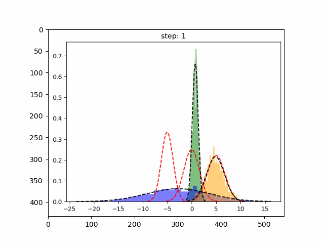
这样就完成了,让我们看看 GMM 表现如何。
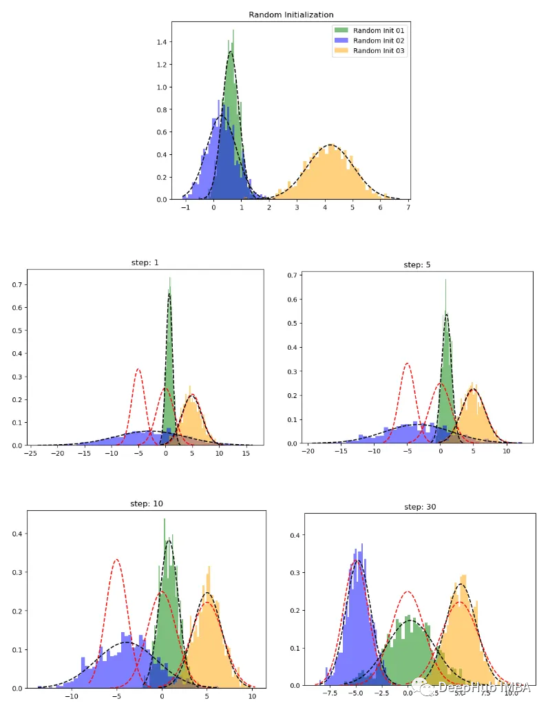
在上图中红色虚线表示原始分布,而其他颜色表示学习分布。 第 30 次迭代后,可以看到的模型在这个生成的数据集上表现良好。
这里只是为了解释GMM的概念进行的Python实现,在实际用例中请不要直接使用,请使用scikit-learn提供的GMM,因为它比我们这个手写的要快多了,具体的对象名是
sklearn.mixture.GaussianMixture
,它的常用参数如下:
- tol:定义模型的停止标准。 当下限平均增益低于 tol 参数时,EM 迭代将停止。
- init_params:用于初始化权重的方法
总结
本文对高斯混合模型进行全面的介绍,希望阅读完本文后你对 GMM 能够有一个详细的了解,GMM 的一个常见问题是它不能很好地扩展到大型数据集。如果你想自己尝试,本文的完整代码在这里:https://github.com/Ransaka/GMM-from-scratch
作者:Ransaka Ravihara