
在本文中将探索各种方法来揭示时间序列数据中的异常模式和异常值。
时间序列数据是按一定时间间隔记录的一系列观测结果。它经常在金融、天气预报、股票市场分析等各个领域遇到。分析时间序列数据可以提供有价值的见解,并有助于做出明智的决策。
异常检测是识别数据中不符合预期行为的模式的过程。在时间序列数据的上下文中,异常可以表示偏离正常模式的重大事件或异常值。检测时间序列数据中的异常对于各种应用至关重要,包括欺诈检测、网络监控和预测性维护。
首先导入库,为了方便数据获取,我们直接使用yfinance:
 import numpy as np
 import pandas as pd
 import matplotlib.pyplot as plt
 import seaborn as sns
 import yfinance as yf

 # Download time series data using yfinance
 data = yf.download('AAPL', start='2018-01-01', end='2023-06-30')
理解时间序列数据
在深入研究异常检测技术之前,先简单介绍时间序列数据的特征。时间序列数据通常具有以下属性:
- 趋势:数据值随时间的长期增加或减少。
- 季节性:以固定间隔重复的模式或循环。
- 自相关:当前观测值与先前观测值之间的相关性。
- 噪声:数据中的随机波动或不规则。
让我们可视化下载的时间序列数据
 # Plot the time series data
 plt.figure(figsize=(12, 6))
 plt.plot(data['Close'])
 plt.xlabel('Date')
 plt.ylabel('Closing Price')
 plt.title('AAPL Stock Price')
 plt.xticks(rotation=45)
 plt.grid(True)

 plt.show()
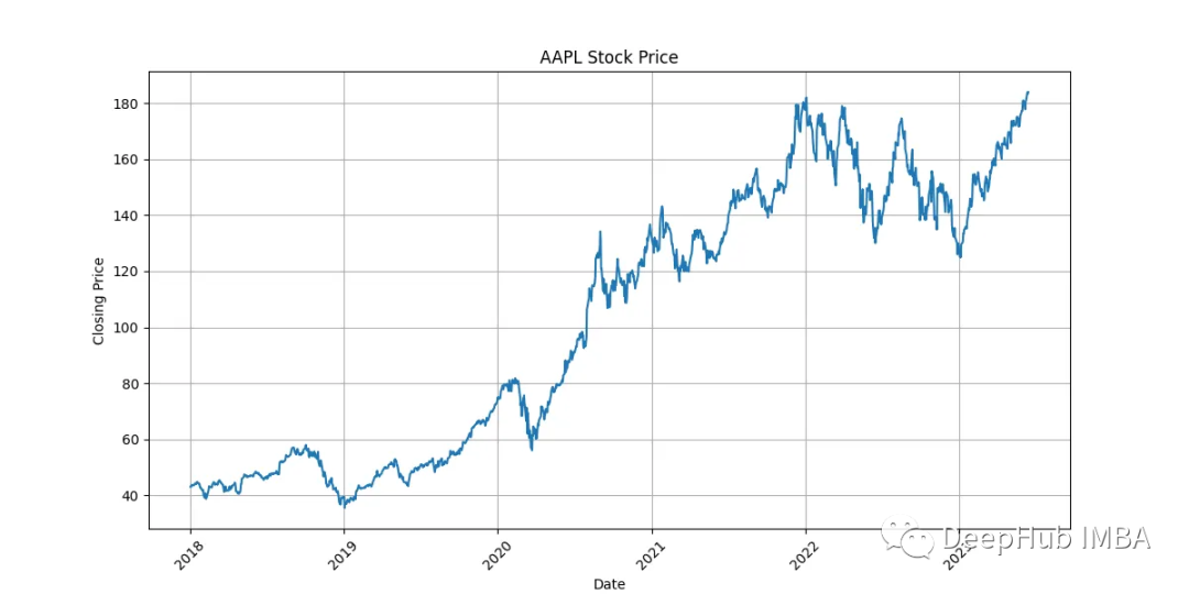
从图中可以观察到股票价格随时间增长的趋势。也有周期性波动,表明季节性的存在。连续收盘价之间似乎存在一些自相关性。
时间序列数据预处理
在应用异常检测技术之前,对时间序列数据进行预处理是至关重要的。预处理包括处理缺失值、平滑数据和去除异常值。
缺失值
由于各种原因,如数据收集错误或数据中的空白,时间序列数据中可能出现缺失值。适当地处理缺失值以避免分析中的偏差是必要的。
 # Check for missing values
 missing_values = data.isnull().sum()
 print(missing_values)
我们使用的股票数据数据不包含任何缺失值。如果存在缺失值,可以通过输入缺失值或删除相应的时间点来处理它们。
平滑数据
对时间序列数据进行平滑处理有助于减少噪声并突出显示潜在的模式。平滑时间序列数据的一种常用技术是移动平均线。
 # Smooth the time series data using a moving average
 window_size = 7
 data['Smoothed'] = data['Close'].rolling(window_size).mean()

 # Plot the smoothed data
 plt.figure(figsize=(12, 6))
 plt.plot(data['Close'], label='Original')
 plt.plot(data['Smoothed'], label='Smoothed')
 plt.xlabel('Date')
 plt.ylabel('Closing Price')
 plt.title('AAPL Stock Price (Smoothed)')
 plt.xticks(rotation=45)
 plt.legend()
 plt.grid(True)

 plt.show()
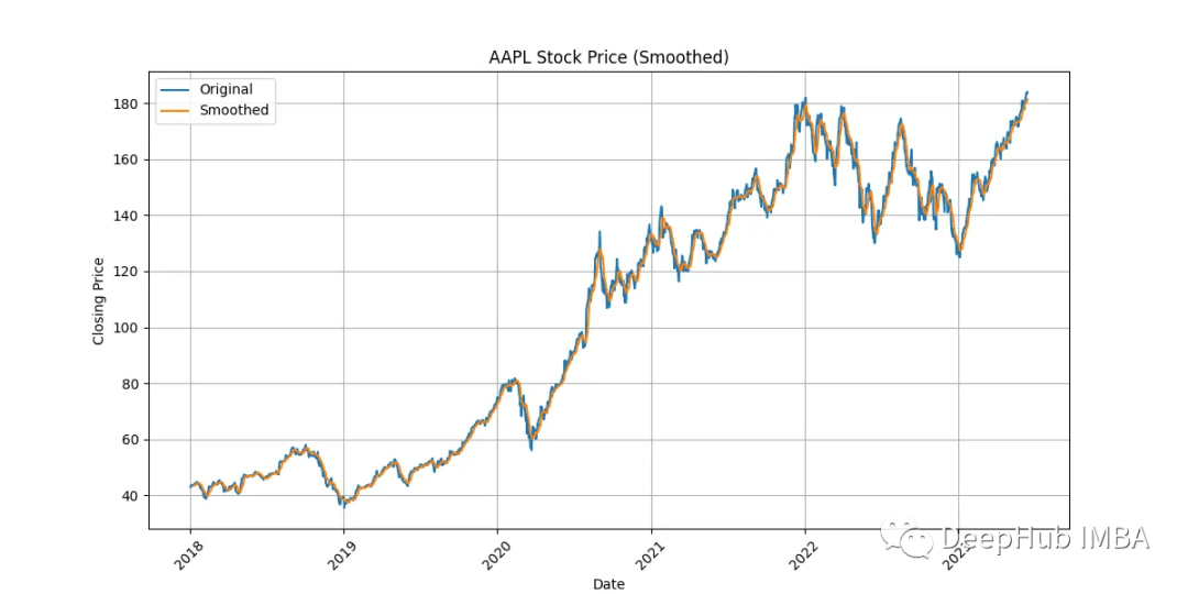
该图显示了原始收盘价和使用移动平均线获得的平滑版本。平滑有助于整体趋势的可视化和减少短期波动的影响。
去除离群值
异常异常值会显著影响异常检测算法的性能。在应用异常检测技术之前,识别和去除异常值是至关重要的。
 # Calculate z-scores for each data point
 z_scores = (data['Close'] - data['Close'].mean()) / data['Close'].std()

 # Define a threshold for outlier detection
 threshold = 3

 # Identify outliers
 outliers = data[np.abs(z_scores) > threshold]

 # Remove outliers from the data
 data = data.drop(outliers.index)

 # Plot the data without outliers
 plt.figure(figsize=(12, 6))
 plt.plot(data['Close'])
 plt.xlabel('Date')
 plt.ylabel('Closing Price')
 plt.title('AAPL Stock Price (Without Outliers)')
 plt.xticks(rotation=45)
 plt.grid(True)

 plt.show()
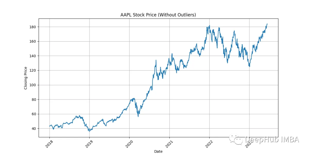
上图显示了去除识别的异常值后的时间序列数据。通过减少极值的影响,去除异常值有助于提高异常检测算法的准确性。
有人会说了,我们不就是要检测异常值吗,为什么要将它删除呢?这是因为,我们这里删除的异常值是非常明显的值,也就是说这个预处理是初筛,或者叫粗筛。把非常明显的值删除,这样模型可以更好的判断哪些难判断的值。
统计方法
统计方法为时间序列数据的异常检测提供了基础。我们将探讨两种常用的统计技术:z-score和移动平均。
z-score
z-score衡量的是观察值离均值的标准差数。通过计算每个数据点的z分数,我们可以识别明显偏离预期行为的观测值。
 # Calculate z-scores for each data point
 z_scores = (data['Close'] - data['Close'].mean()) / data['Close'].std()

 # Plot the z-scores
 plt.figure(figsize=(12, 6))
 plt.plot(z_scores)
 plt.xlabel('Date')
 plt.ylabel('Z-Score')
 plt.title('Z-Scores for AAPL Stock Price')
 plt.xticks(rotation=45)
 plt.axhline(y=threshold, color='r', linestyle='--', label='Threshold')
 plt.axhline(y=-threshold, color='r', linestyle='--')
 plt.legend()
 plt.grid(True)

 plt.show()
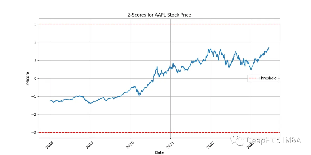
该图显示了每个数据点的计算z-score。z-score高于阈值(红色虚线)的观测值可视为异常。
移动平均线
另一种异常检测的统计方法是基于移动平均线。通过计算移动平均线并将其与原始数据进行比较,我们可以识别与预期行为的偏差。
 # Calculate the moving average
 window_size = 7
 moving_average = data['Close'].rolling(window_size).mean()

 # Calculate the deviation from the moving average
 deviation = data['Close'] - moving_average

 # Plot the deviation
 plt.figure(figsize=(12, 6))
 plt.plot(deviation)
 plt.xlabel('Date')
 plt.ylabel('Deviation')
 plt.title('Deviation from Moving Average')
 plt.xticks(rotation=45)
 plt.axhline(y=0, color='r', linestyle='--', label='Threshold')
 plt.legend()
 plt.grid(True)

 plt.show()
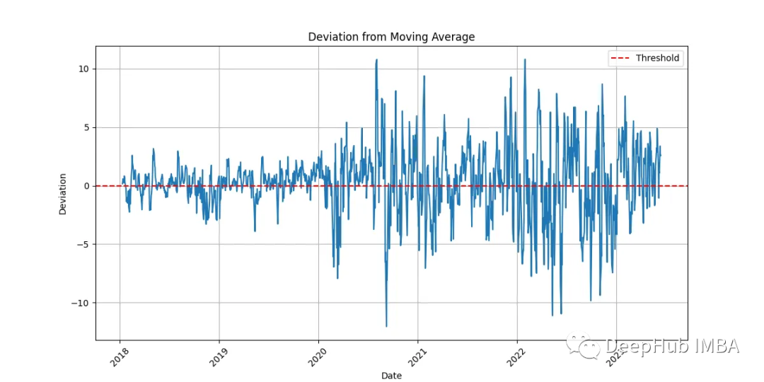
该图显示了每个数据点与移动平均线的偏差。正偏差表示值高于预期行为,而负偏差表示值低于预期行为。
机器学习方法
机器学习方法为时间序列数据的异常检测提供了更先进的技术。我们将探讨两种流行的机器学习算法:孤立森林和LSTM Autoencoder。
孤立森林
孤立森林是一种无监督机器学习算法,通过将数据随机划分为子集来隔离异常。它测量隔离观察所需的平均分区数,而异常情况预计需要更少的分区。
 from sklearn.ensemble import IsolationForest

 # Prepare the data for Isolation Forest
 X = data['Close'].values.reshape(-1, 1)

 # Train the Isolation Forest model
 model = IsolationForest(contamination=0.05)
 model.fit(X)

 # Predict the anomalies
 anomalies = model.predict(X)

 # Plot the anomalies
 plt.figure(figsize=(12, 6))
 plt.plot(data['Close'])
 plt.scatter(data.index, data['Close'], c=anomalies, cmap='cool', label='Anomaly')
 plt.xlabel('Date')
 plt.ylabel('Closing Price')
 plt.title('AAPL Stock Price with Anomalies (Isolation Forest)')
 plt.xticks(rotation=45)
 plt.legend()
 plt.grid(True)

 plt.show()
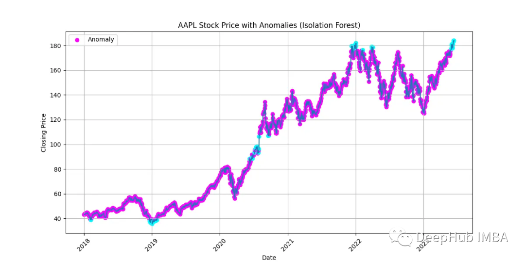
该图显示了由孤立森林算法识别的异常时间序列数据。异常用不同的颜色突出显示,表明它们偏离预期行为。
LSTM Autoencoder
LSTM (Long - Short-Term Memory)自编码器是一种深度学习模型,能够学习时间序列数据中的模式并重构输入序列。通过将重建误差与预定义的阈值进行比较,可以检测异常。
 from tensorflow.keras.models import Sequential
 from tensorflow.keras.layers import LSTM, Dense

 # Prepare the data for LSTM Autoencoder
 X = data['Close'].values.reshape(-1, 1)

 # Normalize the data
 X_normalized = (X - X.min()) / (X.max() - X.min())

 # Train the LSTM Autoencoder model
 model = Sequential([
     LSTM(64, activation='relu', input_shape=(1, 1)),
     Dense(1)
 ])
 model.compile(optimizer='adam', loss='mse')
 model.fit(X_normalized, X_normalized, epochs=10, batch_size=32)

 # Reconstruct the input sequence
 X_reconstructed = model.predict(X_normalized)

 # Calculate the reconstruction error
 reconstruction_error = np.mean(np.abs(X_normalized - X_reconstructed), axis=1)

 # Plot the reconstruction error
 plt.figure(figsize=(12, 6))
 plt.plot(reconstruction_error)
 plt.xlabel('Date')
 plt.ylabel('Reconstruction Error')
 plt.title('Reconstruction Error (LSTM Autoencoder)')
 plt.xticks(rotation=45)
 plt.axhline(y=threshold, color='r', linestyle='--', label='Threshold')
 plt.legend()
 plt.grid(True)

 plt.show()
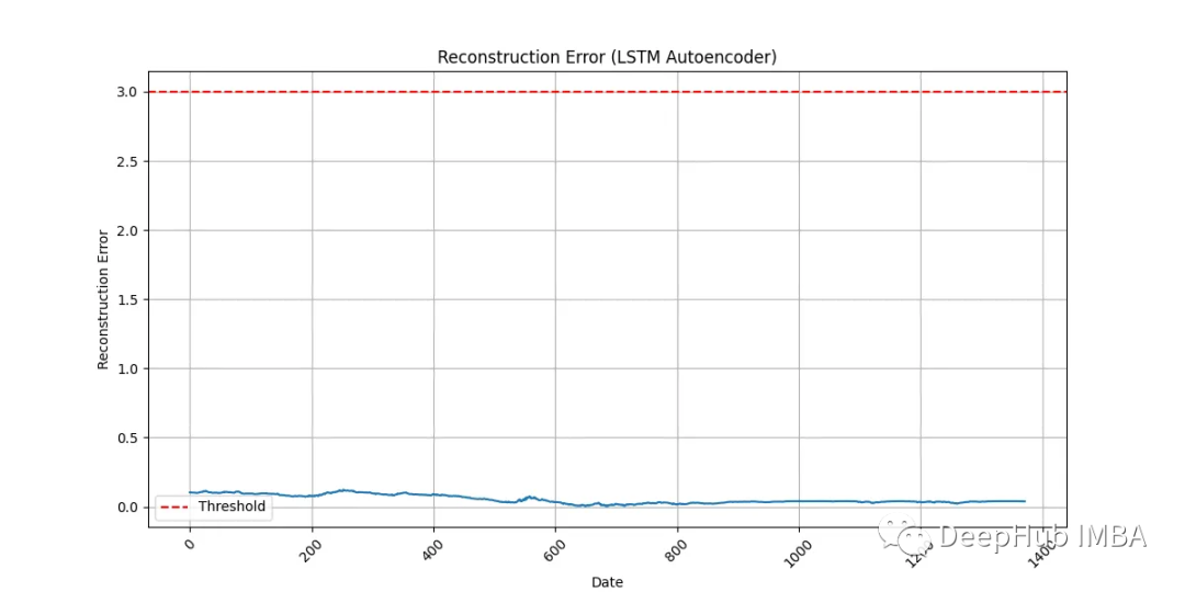
该图显示了每个数据点的重建误差。重建误差高于阈值(红色虚线)的观测值可视为异常。
异常检测模型的评估
为了准确地评估异常检测模型的性能,需要有包含有关异常存在或不存在的信息的标记数据。但是在现实场景中,获取带有已知异常的标记数据几乎不可能,所以可以采用替代技术来评估这些模型的有效性。
最常用的一种技术是交叉验证,它涉及将可用的标记数据分成多个子集或折叠。模型在数据的一部分上进行训练,然后在剩余的部分上进行评估。这个过程重复几次,并对评估结果进行平均,以获得对模型性能更可靠的估计。
当标记数据不容易获得时,也可以使用无监督评估度量。这些指标基于数据本身固有的特征(如聚类或密度估计)来评估异常检测模型的性能。无监督评价指标的例子包括轮廓系数silhouette score、邓恩指数Dunn index或平均最近邻距离。
总结
本文探索了使用机器学习进行时间序列异常检测的各种技术。首先对其进行预处理,以处理缺失值,平滑数据并去除异常值。然后讨论了异常检测的统计方法,如z-score和移动平均。最后探讨了包括孤立森林和LSTM自编码器在内的机器学习方法。
异常检测是一项具有挑战性的任务,需要对时间序列数据有深入的了解,并使用适当的技术来发现异常模式和异常值。记住要尝试不同的算法,微调参数并评估模型的性能,以获得最佳结果。
作者:AI Quant