熟练掌握CV中最基础的概念：图像特征，看这篇万字的长文就够了

目录
1，图像特征
2，角点特征
3，使用OpenCV和PIL进行特征提取和可视化
4，特征匹配
5，图像拼接

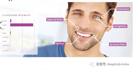
图像特征

什么是图像特征？

**| **特征

·对图像进行描述。

·指出图像中的相关信息。

·将一组图像与其他图像区分开来。

**| **类别

·全局特征：将图像视为一个整体。

·局部特征：图像中的部分区域。

**| **正式定义

在计算机视觉和图像处理中，特征指的是为解决与某一应用有关的计算任务的一段信息。

·所有的机器学习和深度学习算法都依赖于特征。

什么能作为特征？

·单独的像素点强度不能作为特征

**| **特征

·总体强度测量平均值，直方图，调色板等。

·边缘和山脊梯度和轮廓。

·特殊的角点特征和曲率。

·斑点和纹理。

·使用过滤器获得的特征。

例子

1，像素点强度

像素点强度组合作为特征

2，边缘

边缘作为特征

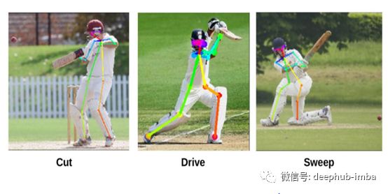
3，关键点

关键点作为特征

什么是好的特征？

那些受外部因素影响不大的特征是好的特征。

**| **特征不变性

·伸缩

·旋转

·转换

·透视法

·仿射

·颜色

·照度

角点特征

·角：定义为两条边的交点。·关键点：图像中具有明确位置且可以可靠检测的点。

**| **适用范围

·运动检测和视频跟踪。·图像注册。·图像拼接和全景拼接。·3D建模和对象识别。

例子

1，关键点

关键点识别

2，角

角识别

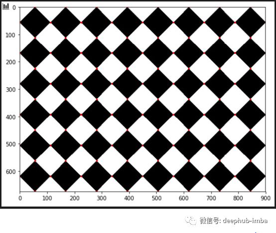
Harris****角点检测

**| **Harris角点检测算法可以分为5个步骤

·转化为灰度图

·计算空间导数

·设置结构向量

·计算Harris响应

·抑制非最大值

| 使用OpenCV实现Harris角点检测

''''' Harris Corners using OpenCV ''' %matplotlib inline  import numpy as np  import cv2  from matplotlib import pyplot as plt  img = cv2.imread("imgs/chapter9/chess_slant.jpg", 1)  #img = cv2.resize(img, (96, 96))  gray = cv2.cvtColor(img,cv2.COLOR_BGR2GRAY)  gray = np.float32(gray)  ################################FOCUS###############################  dst = cv2.cornerHarris(gray,2,3,0.04)  ####################################################################  # Self-study: Parameters  plt.figure(figsize=(8, 8))  plt.imshow(dst, cmap="gray")  plt.show()

'''''  result is dilated for marking the corners '''  dst = cv2.dilate(dst,None)  plt.figure(figsize=(8, 8))  plt.imshow(dst, cmap="gray")  plt.show()

''''' Threshold for an optimal value, it may vary depending on the image.  We first calculate what is the maximum and minimum value of pixel in this image  ''' max_val = np.uint8(dst).max()  min_val = np.uint8(dst).min()  print("max_val = {}".format(max_val))  print("min_val = {}".format(min_val))

输出

max_val = 255  min_val = 0  img = cv2.imread("imgs/chapter9/chess_slant.jpg", 1)  img[dst>0.1*dst.max()]=[0,0,255]  plt.figure(figsize=(8, 8))  plt.imshow(img[:,:,::-1])  plt.show()

|利用OpenCV-harris角点求角点坐标

%matplotlib inline  import numpy as np  import cv2  from matplotlib import pyplot as plt   img = cv2.imread("imgs/chapter9/chess_slant.jpg", 1);  #img = cv2.resize(img, (96, 96))  gray = cv2.cvtColor(img,cv2.COLOR_BGR2GRAY)  # find Harris corners  gray = np.float32(gray)  dst = cv2.cornerHarris(gray,2,3,0.04)  dst = cv2.dilate(dst,None)  ret, dst = cv2.threshold(dst,0.01*dst.max(),255,0)  dst = np.uint8(dst)  # find centroids  ret, labels, stats, centroids = cv2.connectedComponentsWithStats(dst)  # define the criteria to stop and refine the corners  # Explain Criteria  criteria = (cv2.TERM_CRITERIA_EPS + cv2.TERM_CRITERIA_MAX_ITER, 100, 0.001)  corners = cv2.cornerSubPix(gray,np.float32(centroids),(5,5),(-1,-1),criteria)  # Now draw them  res = np.hstack((centroids,corners))  res = np.int0(res)  for x1, y1, x2, y2 in res:      #cv2.circle(img,(x1, y1), 5, (0,255,0), -1) # Point Centroids     cv2.circle(img,(x2, y2), 10, (0,0,255), -1) # Point corners  #img[res[:,1],res[:,0]]=[0,0,255]  #img[res[:,3],res[:,2]] = [0,255,0]  plt.figure(figsize=(8, 8))  plt.imshow(img[:,:,::-1])  plt.show()

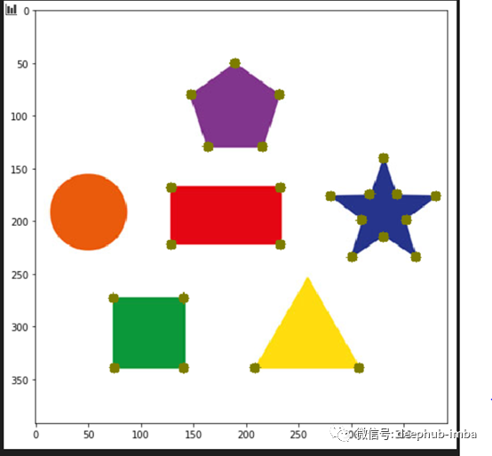
**Shi-Tomasi **角点检测

·Harris角点检测有一个角点选择准则。

·为每个像素计算一个分数，如果分数高于某个值，则将该像素标记为角点。

·Shi和Tomasi建议取消这项功能。只有特征值可以用来检查像素是否是角点。

·这些角点是对harris角点的一次升级。

%matplotlib inline  import numpy as np  import cv2   from matplotlib import pyplot as plt  img = cv2.imread("imgs/chapter9/shape.jpg", 1)  gray = cv2.cvtColor(img,cv2.COLOR_BGR2GRAY)  ################################FOCUS###############################  corners = cv2.goodFeaturesToTrack(gray,25,0.01,10)  # Self-study: Parameters  corners = np.int0(corners)  ####################################################################  ################################FOCUS###############################  for i in corners:       x,y = i.ravel()       cv2.circle(img,(x,y), 5,(0, 125, 125),-1)  ################################################################  plt.figure(figsize=(8, 8))  plt.imshow(img[:,:,::-1])  plt.show()

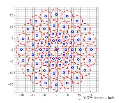
OpenCV****快速角点检测

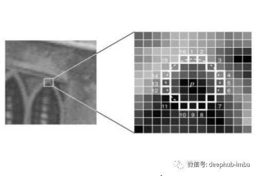
·选择一个像素，让它的强度为i。

·选择阈值t。

·如上图所示，在像素周围画一个16像素的圆。

·现在，如果圆中存在一组n个连续像素（16个像素），且这些像素都比i+t强度更大，或者都比i-t强度更小，则像素p是一个角点。

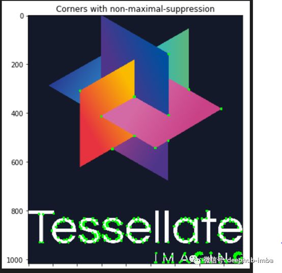
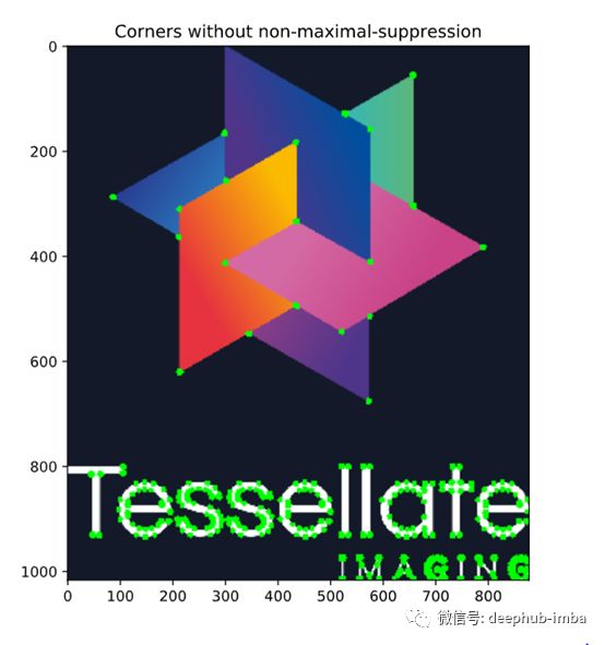
import cv2  from matplotlib import pyplot as plt  img = cv2.imread('imgs/chapter9/tessellate.png',1)  img2 = img.copy()  img3 = img.copy()  ###############################FOCUS################################   # Initiate FAST object with default values  fast = cv2.FastFeatureDetector_create()  # find and draw the keypoints  kp = fast.detect(img,None)  ####################################################################  for i in kp:      x,y = int(i.pt[0]), int(i.pt[1])      cv2.circle(img2,(x,y), 5,(0, 255, 0),-1)  # Print all default params  print ("Threshold: ", fast.getThreshold())  print ("nonmaxSuppression: ", fast.getNonmaxSuppression())  print ("neighborhood: ", fast.getType())  print ("Total Keypoints with nonmaxSuppression: ", len(kp))  # Disable nonmaxSuppression  fast.setNonmaxSuppression(0)  kp = fast.detect(img,None)  print ("Total Keypoints without nonmaxSuppression: ", len(kp))  for i in kp:      x,y = int(i.pt[0]), int(i.pt[1])      cv2.circle(img3,(x,y), 5,(0, 255, 0),-1)  f = plt.figure(figsize=(15,15))  f.add_subplot(2, 1, 1).set_title('Corners with non-maximal-suppression')  plt.imshow(img2[:, :,::-1])  f.add_subplot(2, 1, 2).set_title('Corners without non-maximal-suppression')  plt.imshow(img3[:, :,::-1])  plt.show()

输出

Threshold:  10   nonmaxSuppression:  True   neighborhood:  2   Total Keypoints with nonmaxSuppression:  225   Total Keypoints without nonmaxSuppression:  1633

使用OpenCV和PIL进行特征提取和可视化

A级特征

HoG features（方向梯度直方图特征）

梯度直方图
用于目标检测

步骤

查找x和y方向上的梯度
使用梯度大小和方向将梯度归类为直方图。

HoG特征对图像中物体的旋转很敏感。

使用Skimage来实现HoG

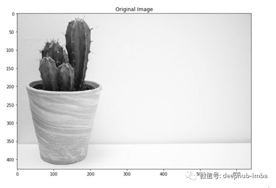
%matplotlib inlineimport numpy as npimport skimageimport skimage.featureimport cv2from matplotlib import pyplot as pltimg = cv2.imread("imgs/chapter9/plant.jpg", 1)features, output = skimage.feature.hog(img, orientations=9, pixels_per_cell=(8,8),cells_per_block=(3, 3), block_norm='L2-Hys',visualize=True,transform_sqrt=False, feature_vector=True,multichannel=None)print(features.shape)# Rescale histogram for betterdisplayoutput = skimage.exposure.rescale_intensity(output, in_range=(0, 10))f =plt.figure(figsize=(15,15))f.add_subplot(2, 1, 1).set_title('Original Image')plt.imshow(img[:, :,::-1])f.add_subplot(2, 1, 2).set_title('Features')plt.imshow(output)plt.show()

输出

(322218,)

Daisy Features（面向稠密特征提取的可快速计算的局部图像特征描述子）

升级版的HOG特征
创建一个不适合可视化的稠密特征向量

步骤

T块->计算梯度或梯度直方图
S块->使用高斯加权加法（轮廓）组合T块特征
N块->归一化添加的特征（使范围在0-1之间）
D块->缩小特征维数（PCA算法）
Q块->压缩特征用于存储

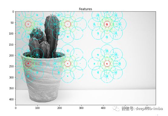
使用Sklearn实现面向稠密特征提取的可快速计算的局部图像特征描述子

import numpyasnpimport skimageimport skimage.featureimport cv2
from matplotlibimport pyplot as pltimg = cv2.imread("imgs/chapter9/plant.jpg", 0)#img = cv2.resize(img, (img.shape[0]//4,img.shape[1]//4))features, output = skimage.feature.daisy(img, step=180, radius=58, rings=2, histograms=8, orientations=9, visualize=True)print(features.shape)f = plt.figure(figsize=(15,15))f.add_subplot(2, 1, 1).set_title('Original Image');plt.imshow(img, cmap="gray")f.add_subplot(2, 1, 2).set_title('Features');plt.imshow(output);plt.show()

输出

(2, 3, 153)

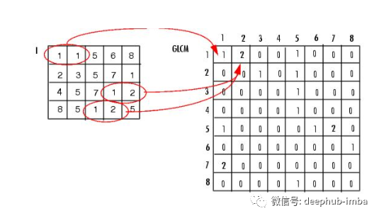
GLCM Features（灰度共生矩阵特征）

灰度协方差矩阵
计算各像素在不同方面(同质性、均匀性)的整体平均相关程度。
灰度共生矩阵(GLCM)通过计算灰度像素i与j在特定空间关系中出现的频率。

使用Skimage实现GLCM

*'''**

* Source: https://scikitimage.org/docs/dev/auto_examples/features_detection/plot_glcm.html**'''**import****matplotlib.pyplot****as****plt**

from skimage.featureimport greycomatrix, greycoprops
from skimageimport data
PATCH_SIZE = 21

# open the camera image
image = data.camera()

# select some patches from grassy areas of the image
grass_locations = [(474, 291), (440, 433), (466, 18), (462, 236)]
grass_patches = []
for loc ingrass_locations:
    grass_patches.append(image[loc[0]:loc[0] + PATCH_SIZE,
                               loc[1]:loc[1] + PATCH_SIZE])

# select some patches from sky areas of the image
sky_locations = [(54, 48), (21, 233), (90, 380), (195, 330)]
sky_patches = []
for loc insky_locations:
    sky_patches.append(image[loc[0]:loc[0] + PATCH_SIZE,
                             loc[1]:loc[1] + PATCH_SIZE])

# compute some GLCM properties each patch
xs = []
ys = []
for patch in (grass_patches + sky_patches):
    glcm = greycomatrix(patch, [5], [0], 256, symmetric=True, normed=True)
    xs.append(greycoprops(glcm, 'dissimilarity')[0, 0])
    ys.append(greycoprops(glcm, 'correlation')[0, 0])
# create the figure
fig = plt.figure(figsize=(8, 8))

# display original image with locations of patches
ax = fig.add_subplot(3, 2, 1)
ax.imshow(image, cmap=plt.cm.gray, interpolation='nearest',
          vmin=0, vmax=255)
for (y, x) ingrass_locations:
    ax.plot(x + PATCH_SIZE / 2, y + PATCH_SIZE / 2, 'gs')
for (y, x) insky_locations:
    ax.plot(x + PATCH_SIZE / 2, y + PATCH_SIZE / 2, 'bs')
ax.set_xlabel('Original Image')
ax.set_xticks([])
ax.set_yticks([])
ax.axis('image')

# for each patch, plot (dissimilarity, correlation)
ax = fig.add_subplot(3, 2, 2)
ax.plot(xs[:len(grass_patches)], ys[:len(grass_patches)], 'go',
        label='Grass')
ax.plot(xs[len(grass_patches):], ys[len(grass_patches):], 'bo',
        label='Sky')
ax.set_xlabel('GLCM Dissimilarity')
ax.set_ylabel('GLCM Correlation')
ax.legend()

# display the image patchesfor i, patch in enumerate(grass_patches):
    ax = fig.add_subplot(3, len(grass_patches), len(grass_patches)*1 + i + 1)
    ax.imshow(patch, cmap=plt.cm.gray, interpolation='nearest',
              vmin=0, vmax=255)
    ax.set_xlabel('Grass %d' % (i + 1))

for i, patch in enumerate(sky_patches):
    ax = fig.add_subplot(3, len(sky_patches), len(sky_patches)*2 + i + 1)
    ax.imshow(patch, cmap=plt.cm.gray, interpolation='nearest',
              vmin=0, vmax=255)
    ax.set_xlabel('Sky %d' % (i + 1))

# display the patches and plotfig.suptitle('Grey level co-occurrence matrix features', fontsize=14)
plt.show()

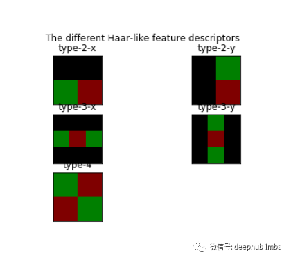
HAAR Features（哈尔特征）

用于物体识别

哈尔矩形特征

矩形内区域像素之和的差值。
每个特征都是一个单独的值，由白色矩形下的像素之和减去黑色矩形下的像素之和得到。

* *

*'''**

*Source:*

*https://scikitimage.org/docs/dev/auto_examples/features_detection/plot_haar.html**

''' *# Haar like feature Descriptors*

importnumpyasnp
importmatplotlib.pyplotasplt
importskimage.feature
fromskimage.featureimport haar_like_feature_coord, draw_haar_like_feature 
images = [np.zeros((2, 2)), np.zeros((2, 2)),np.zeros((3, 3)), np.zeros((3, 3)),np.zeros((2, 2))] 
feature_types = ['type-2-x', 'type-2-y','type-3-x', 'type-3-y',                  'type-4'] 
fig, axs = plt.subplots(3, 2)
for ax, img, feat_t inzip(np.ravel(axs), images, feature_types):
    coord, _ = haar_like_feature_coord(img.shape[0],
                                       img.shape[1],
                                       feat_t)    
    haar_feature = draw_haar_like_feature(img, 0, 0,       img.shape[0],img.shape[1],coord,max_n_features=1,                       random_state=0)    
    ax.imshow(haar_feature)    
    ax.set_title(feat_t)    
    ax.set_xticks([])    
    ax.set_yticks([])  fig.suptitle('The different Haar-like feature descriptors') plt.axis('off')
plt.show()

LBP Features（局部二值模式特征）

局部二值模式

要素

LBP阈值
特征求和

import numpyas npimport skimageimport skimage.featureimport cv2from matplotlib import pyplot as pltimg = cv2.imread("imgs/chapter9/plant.jpg", 0);#img = cv2.resize(img,(img.shape[0]//4,img.shape[1]//4));
output = skimage.feature.local_binary_pattern(img, 3, 8, method='default')print(features.shape);
# Rescale histogram for betterdisplay#output = skimage.exposure.rescale_intensity(output,in_range=(0, 10))

f = plt.figure(figsize=(15,15))f.add_subplot(2, 1, 1).set_title('Original Image');plt.imshow(img, cmap="gray")f.add_subplot(2, 1, 2).set_title('Features');plt.imshow(output);plt.show()

输出

(2,3, 153)

Blobs as features（斑点作为特征）

Blob检测方法的目的是检测数字图像中与周围区域相比具有不同属性(如亮度或颜色)的区域。
通俗地说，blob是图像的一个区域，其中一些属性是常量或近似常量，可以认为blob中的所有点在某种意义上是相似的。

使用Skimage来实现Blobs

import numpyas npimport skimageimport skimage.featureimport cv2import mathfrom matplotlib import pyplot as plt
img = cv2.imread("imgs/chapter9/shape.jpg", 0)#img =skimage.data.hubble_deep_field()[0:500, 0:500]#image_gray =skimage.color.rgb2gray(image)
blobs = skimage.feature.blob_dog(img, max_sigma=5, threshold=0.05)
blobs[:, 2] = blobs[:, 2]print(blobs.shape)
for y , x, r in blobs:cv2.circle(img,(int(x), int(y)), int(r), (0,255,0), 1)

f = plt.figure(figsize=(15,15))f.add_subplot(2, 1, 1).set_title('OriginalImage');plt.imshow(img, cmap="gray")plt.show()

输出

(91, 3)

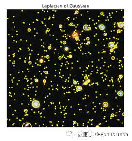
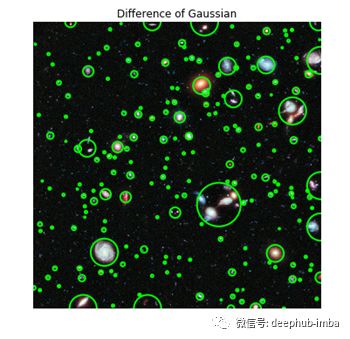
使用Blobs检测外太空星系

'''

Source:

https://scikitimage.org/docs/dev/auto_examples/features_detection/plot_blob.html

'''

from mathimport sqrtfromskimage import datafromskimage.feature import blob_dog, blob_log, blob_dohfromskimage.color import rgb2grayimportmatplotlib.pyplot as pltimage =data.hubble_deep_field()[0:500, 0:500]image_gray= rgb2gray(image)blobs_log= blob_log(image_gray, max_sigma=30, num_sigma=10, threshold=.1)# Computeradii in the 3rd column.blobs_log[:,2] = blobs_log[:, 2] * sqrt(2)blobs_dog= blob_dog(image_gray, max_sigma=30, threshold=.1)blobs_dog[:,2] = blobs_dog[:, 2] * sqrt(2)blobs_doh= blob_doh(image_gray, max_sigma=30, threshold=.01)blobs_list= [blobs_log, blobs_dog, blobs_doh]colors =['yellow', 'lime', 'red']titles =['Laplacian of Gaussian', 'Difference of Gaussian',          'Determinant of Hessian']sequence= zip(blobs_list, colors, titles)fig, axes= plt.subplots(3, 1, figsize=(15, 15), sharex=True, sharey=True)ax =axes.ravel()for idx,(blobs, color, title) in enumerate(sequence):    ax[idx].set_title(title)    ax[idx].imshow(image,interpolation='nearest')    for blob in blobs:        y, x, r = blob        c = plt.Circle((x, y), r, color=color,linewidth=2, fill=False)        ax[idx].add_patch(c)    ax[idx].set_axis_off()plt.tight_layout()plt.show()

B****级特征

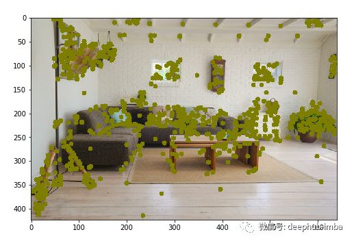
SIFT Features（尺度不变特征变换特征）

尺度不变特征变换
专利持有人是加拿大的UBC大学

SIFT具有特征如下：

尺度不变性（图像尺度变化，提取的特征不变）
旋转不变性（图像旋转，提取的特征不变）
亮度不变性（亮度发生改变，提取的特征不变）
视角不变性（视角变化，提取的特征不变）

SIFT提取步骤

构建规模空间金字塔
使用近似LOG算子处理特征和梯度
在高斯图像的差分中找出最大和最小的关键点。
剔除非关键点
给关键点分配一个方向。
生成最终的SIFT特征—为缩放和旋转不变性生成一个新的表示。

使用OpenCV实现SIFT

'''
NOTE: Patented work. Cannot be used for commercial purposes1.pip installopencv-contrib-python==3.4.2.16
2.pip install opencv-python==3.4.2.16
'''

import numpy as npimport cv2print(cv2.__version__)from matplotlib import pyplot as pltimg = cv2.imread("imgs/chapter9/indoor.jpg", 1);
gray = cv2.cvtColor(img,cv2.COLOR_BGR2GRAY)
sift = cv2.xfeatures2d.SIFT_create()keypoints, descriptors = sift.detectAndCompute(gray, None)

for i in keypoints:    x,y = int(i.pt[0]), int(i.pt[1])    cv2.circle(img,(x,y), 5,(0, 125,125),-1)
plt.figure(figsize=(8, 8))plt.imshow(img[:,:,::-1]);plt.show()

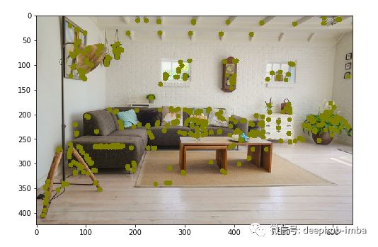
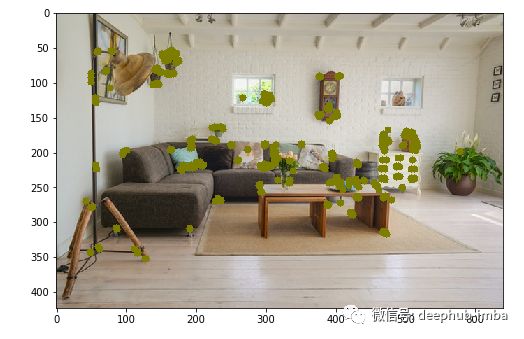
CenSurE Features（中心环绕特征）

中心环绕用于实时特征检测
胜过许多其他关键点检测器和特征提取器。

CenSureE具有特征如下：

尺度不变性（图像尺度变化，提取的特征不变）
旋转不变性（图像旋转，提取的特征不变）
亮度不变性（亮度发生改变，提取的特征不变）
视角不变性（视角变化，提取的特征不变）

使用Skimage实现CENSURE

import numpyas npimport cv2import skimage.featurefrom matplotlib import pyplot as pltimg = cv2.imread("imgs/chapter9/indoor.jpg", 1);
gray = cv2.cvtColor(img,cv2.COLOR_BGR2GRAY)
detector = skimage.feature.CENSURE(min_scale=1, max_scale=7, mode='Star',non_max_threshold=0.05, line_threshold=10)
detector.detect(gray)
for i in detector.keypoints:x,y = int(i[1]), int(i[0])cv2.circle(img,(x,y), 5,(0, 125, 125),-1)
plt.figure(figsize=(8, 8))plt.imshow(img[:,:,::-1]);plt.show()

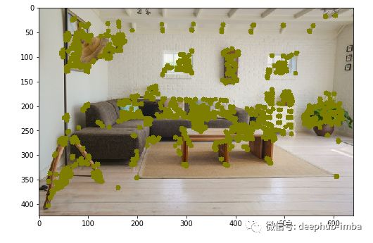
SURFFeatures（快速鲁棒特征）

快速鲁棒特征
已获得专利的局部特征检测器和特征描述子
标准版本的SURF比SIFT要快好几倍

SURF使用的算法：

Hessian斑点检测器行列式的整数近似值
Haar小波响应之和
多分辨率金字塔

SUFR特性有：

尺度不变性（图像尺度变化，提取的特征不变）
旋转不变性（图像旋转，提取的特征不变）
视角不变性（视角变化，提取的特征不变）

* *

*'''**

*NOTE: Patented work. Cannot be used for commercial purposes**

*

*1.pip install opencv-contrib-python==3.4.2.16**

*2.pip install opencv-python==3.4.2.16*

import numpy as np
importcv2
frommatplotlibimport pyplot as plt
img = cv2.imread("imgs/chapter9/indoor.jpg", 1);

gray = cv2.cvtColor(img,cv2.COLOR_BGR2GRAY)

surf = cv2.xfeatures2d.SURF_create(1000)
keypoints, descriptors = surf.detectAndCompute(gray, None)

for i in keypoints:
    x,y = int(i.pt[0]), int(i.pt[1])
    cv2.circle(img,(x,y), 5,(0, 125, 125),-1)

plt.figure(figsize=(8, 8))
plt.imshow(img[:,:,::-1]);
plt.show()

BRIEF Features（二进制鲁棒独立的基本特征）

二进制鲁棒的独立基本特征
在很多情况下，在速度和识别率方面都优于其他快速描述子，如SURF和SIFT。

步骤：

使用高斯核平滑图像
转换为二进制特征向量

使用Opencv实现BRIEF

import numpyas npimport cv2from matplotlib import pyplot as pltimg = cv2.imread("imgs/chapter9/indoor.jpg", 1);
gray = cv2.cvtColor(img,cv2.COLOR_BGR2GRAY)
# Initiate FAST detectorstar = cv2.xfeatures2d.StarDetector_create()kp = star.detect(gray,None)
brief = cv2.xfeatures2d.BriefDescriptorExtractor_create()keypoints, descriptors = brief.compute(gray, kp)

for i in keypoints:x,y = int(i.pt[0]), int(i.pt[1])cv2.circle(img,(x,y), 5,(0, 125, 125),-1)
plt.figure(figsize=(8, 8))plt.imshow(img[:,:,::-1]);plt.show()

BRISK Features（二进制鲁棒不变可扩展关键点特征）

（Binary RobustIndependent Elementary Features.）原文给的这个但BRISK全称应该是Binary Robust Invariant Scalable Keypoints

由三部分组成

采样模式：在描述子周围的位置采样

方向补偿:对关键点的方向和旋转进行某种机制的补偿。
抽样对:构建最终描述符时要比较哪些对。

import numpy as npimport cv2from matplotlib import pyplot as pltimg = cv2.imread("imgs/chapter9/indoor.jpg", 1);
gray = cv2.cvtColor(img,cv2.COLOR_BGR2GRAY)
brisk = cv2.BRISK_create()keypoints, descriptors = brisk.detectAndCompute(gray, None)
for i in keypoints:x,y = int(i.pt[0]), int(i.pt[1])cv2.circle(img,(x,y), 5,(0, 125, 125),-1)
plt.figure(figsize=(8, 8))plt.imshow(img[:,:,::-1]);plt.show()

KAZE and Accelerated-KAZE features（KAZE是日语风的谐音）

使用OpenCV实现KAZE

import numpyas npimport cv2from matplotlib import pyplot as pltimg = cv2.imread("imgs/chapter9/indoor.jpg", 1);
gray = cv2.cvtColor(img,cv2.COLOR_BGR2GRAY)
kaze = cv2.KAZE_create()keypoints, descriptors = kaze.detectAndCompute(gray, None)
for i in keypoints:x,y = int(i.pt[0]), int(i.pt[1])cv2.circle(img,(x,y), 5,(0, 125, 125),-1)
plt.figure(figsize=(8, 8))plt.imshow(img[:,:,::-1]);plt.show()

AKAZE Features

使用OpenCV实现AKAZE

import numpyas npimport cv2from matplotlib import pyplot as pltimg = cv2.imread("imgs/chapter9/indoor.jpg", 1);
gray = cv2.cvtColor(img,cv2.COLOR_BGR2GRAY)
akaze = cv2.AKAZE_create()keypoints, descriptors = akaze.detectAndCompute(gray, None)
for i in keypoints:x,y = int(i.pt[0]), int(i.pt[1])cv2.circle(img,(x,y), 5,(0, 125, 125),-1)
plt.figure(figsize=(8, 8))plt.imshow(img[:,:,::-1]);plt.show()

ORB Features

面向快速鲁棒的BRIEF特征

使用OpenCV实现Orb

import numpyas npimport cv2from matplotlib import pyplot as pltimg = cv2.imread("imgs/chapter9/indoor.jpg", 1)
gray = cv2.cvtColor(img,cv2.COLOR_BGR2GRAY)
orb = cv2.ORB_create(500)keypoints, descriptors = orb.detectAndCompute(gray, None)
for i in keypoints:x,y = int(i.pt[0]), int(i.pt[1])cv2.circle(img,(x,y), 5,(0, 125, 125),-1)
plt.figure(figsize=(8, 8))plt.imshow(img[:,:,::-1])plt.show()

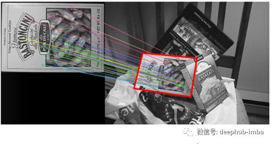
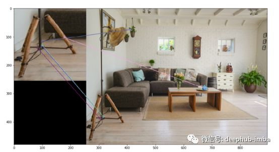
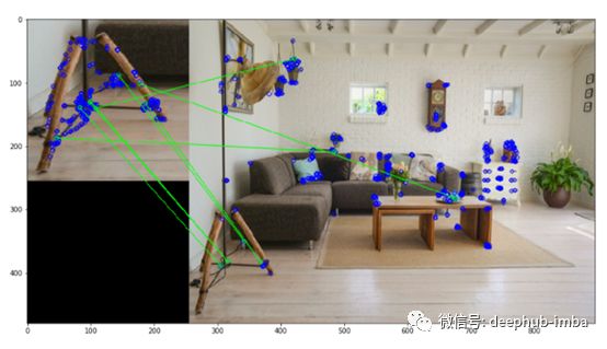
特征匹配

用于识别多幅图像中的相似特征。
用于目标检测。

方法

1.暴力算法

将图像1中的每个特征与图像2中的每个特征逐个进行匹配

2.基于FLANN（快速最近邻开源库）的匹配

快速最近邻开源库
它包含一组算法，这些算法针对大型数据集中的快速最近邻搜索和高维特征进行了优化。

使用Opencv实现特征匹配

'''*
Using Brute-Force matching*
'''

import numpy as npimport cv2from matplotlib import pyplot as plt
orb = cv2.ORB_create(500)
img1 = cv2.imread("imgs/chapter9/indoor_lamp.jpg", 1);img1 = cv2.resize(img1, (256, 256));gray1 = cv2.cvtColor(img1,cv2.COLOR_BGR2GRAY);
img2 = cv2.imread("imgs/chapter9/indoor.jpg", 1);img2 = cv2.resize(img2, (640, 480));gray2 = cv2.cvtColor(img2,cv2.COLOR_BGR2GRAY);
# find the keypoints anddescriptors with SIFTkp1, des1 = orb.detectAndCompute(img1,None)kp2, des2 = orb.detectAndCompute(img2,None)
# BFMatcher with default paramsbf = cv2.BFMatcher()matches = bf.knnMatch(des1,des2,k=2)
# Apply ratio testgood = []for m,n in matches:if m.distance< 0.75*n.distance:good.append([m])
# cv.drawMatchesKnn expects list oflists as matches.img3 = cv2.drawMatchesKnn(img1,kp1,img2,kp2,good,None,flags=cv2.DrawMatchesFlags_NOT_DRAW_SINGLE_POINTS)
plt.figure(figsize=(15, 15))plt.imshow(img3[:,:,::-1])plt.show()

使用Opencv实现基于Flann特征匹配

*'''**

*Using Flann-based matching on ORB features**

import numpy as np
import cv2
from matplotlibimport pyplot as plt
import imutils

orb = cv2.ORB_create(500)

img1 = cv2.imread("imgs/chapter9/indoor_lamp.jpg", 1);
img1 = cv2.resize(img1, (256, 256));
gray1 = cv2.cvtColor(img1,cv2.COLOR_BGR2GRAY);

img2 = cv2.imread("imgs/chapter9/indoor.jpg", 1);
img2 = cv2.resize(img2, (640, 480));
gray2 = cv2.cvtColor(img2,cv2.COLOR_BGR2GRAY);

# find the keypoints and descriptors with SIFT
kp1, des1 = orb.detectAndCompute(img1,None)
kp2, des2 = orb.detectAndCompute(img2,None)

# FLANN parameters
FLANN_INDEX_LSH = 6
index_params= dict(algorithm = FLANN_INDEX_LSH,
                   table_number = 6, # 12
                   key_size = 12,     # 20
                   multi_probe_level = 1) #2
search_params = dict(checks=50)   # or pass empty dictionary
flann = cv2.FlannBasedMatcher(index_params,search_params)
matches = flann.knnMatch(des1,des2,k=2)
# Need to draw only good matches, so create a mask
matchesMask = [[0,0] for i in range(len(matches))]
# ratio test as per Lowe's paperfor i,(m,n) in enumerate(matches):
    if m.distance < 0.7*n.distance:
        matchesMask[i]=[1,0]
draw_params = dict(matchColor = (0,255,0),
                   singlePointColor = (255,0,0),
                   matchesMask = matchesMask,
                   flags = cv2.DrawMatchesFlags_DEFAULT)
img3 = cv2.drawMatchesKnn(img1,kp1,img2,kp2,matches,None,**draw_params)

plt.figure(figsize=(15, 15))
plt.imshow(img3[:,:,::-1])
plt.show()

图像拼接

图像拼接或照片拼接是将多个摄影图像中重叠的视野相结合，产生一个分段的全景图或高分辨率图像的过程。

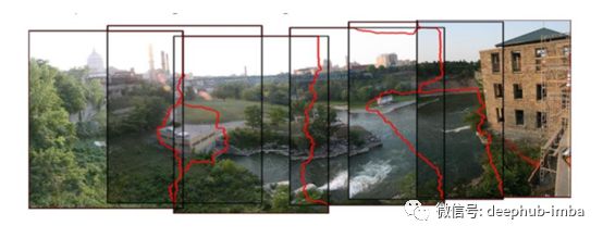
使用OpenCV来实现图像拼接

from matplotlib import pyplot as plt

%matplotlib inline

import cv2

import numpy as np

import argparse

import sys

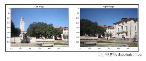
modes = (cv2.Stitcher_PANORAMA, cv2.Stitcher_SCANS)# read input imagesimgs = [cv2.imread("imgs/chapter9/left.jpeg", 1),cv2.imread("imgs/chapter9/right.jpeg", 1)]stitcher = cv2.Stitcher.create(cv2.Stitcher_PANORAMA)

status, pano = stitcher.stitch(imgs)f = plt.figure(figsize=(15,15))

f.add_subplot(1, 2, 1).set_title('Left Image')

plt.imshow(imgs[0][:,:,::-1])

f.add_subplot(1, 2, 2).set_title('Right Image')

plt.imshow(imgs[1][:,:,::-1])

plt.show()

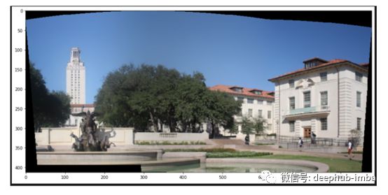
plt.figure(figsize=(15, 15))plt.imshow(pano[:,:,::-1])plt.show()

作者：Abhishek和Akash

deephub翻译组：tensor-zhang，gkkkkkk

DeepHub

微信号 : deephub-imba

每日大数据和人工智能的重磅干货

大厂职位内推信息

长按识别二维码关注 ->

好看就点在看！********** **********

标签：

熟练掌握CV中最基础的概念：图像特征，看这篇万字的长文就够了

发表评论

“熟练掌握CV中最基础的概念：图像特征，看这篇万字的长文就够了”的评论:

关于作者

Deephub

相关阅读

文章导航