自动驾驶规划 - Apollo Lattice Planner算法【1】

文章目录

Lattice Planner简介

LatticePlanner算法属于一种局部轨迹规划器，输出轨迹将直接输入到控制器，由控制器完成对局部轨迹的跟踪控制。因此，Lattice Planner输出的轨迹是一条光滑无碰撞满足车辆运动学约束和速度约束的平稳安全的局部轨迹。Lattice Planner的输入端主要由三部分组成，感知及障碍物信息、参考线信息及定位信息。局部规划模块的输出是带有速度信息的一系列轨迹点组成的轨迹，其保证了车辆控制器在车辆跟踪控制过程中的平稳性和安全性。挺复杂的越挖越多，看来得慢慢总结了（主要为了学思路，总结到自己的项目中）。

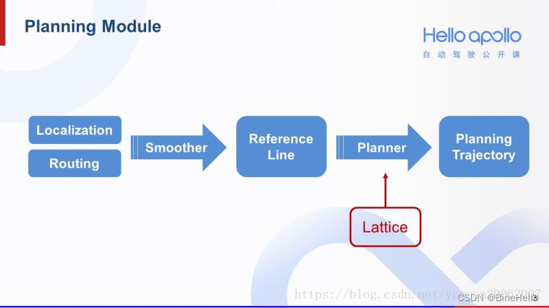
局部规划模块的输出是带有速度信息(速度信息哪里来的？)的一系列轨迹点组成的轨迹，其保证了车辆控制器在车辆跟踪控制过程中的平稳性和安全性。下面讲一下Apollo中的Lattice Planner的算法过程和代码解析。《刚学，写得可能不好，大佬们评论区指正😭😭》

Lattice Planner 算法思路

1. 离散化参考线的点
2. 在参考线上计算匹配点
3. 根据匹配点，计算Frenet坐标系的S-L值
4. 计算障碍物的s-t图
5. 生成横纵向采样路径
6. 计算cost值，进行碰撞检测
7. 优先选择cost最小的轨迹且不碰撞的轨迹

在整体Apollo代码的结构，Lattice Planner的主要思路和实现是在Plan里面的PlanOnReferenceLine中，如下。

Status LatticePlanner::Plan(const TrajectoryPoint& planning_start_point,Frame* frame, ADCTrajectory* ptr_computed_trajectory){...auto status =PlanOnReferenceLine(planning_start_point, frame,&reference_line_info);//主要是逻辑在这个函数里面...}

PlanOnReferenceLine 主要是7步，按照上面的算法逻辑解析。

1. 离散化参考线的点

作为Lattice Planner的第一步，这部分的主要做的是将reference_line上的点，一个个搬到path_points中，其中增加了计算起点到当前点的累积距离s，s的主要作用是为S-L坐标系使用。

// 1. 离散化参考线的点（obtain a reference line and transform it to the PathPoint format）auto ptr_reference_line =
      std::make_shared<std::vector<PathPoint>>(ToDiscretizedReferenceLine(
          reference_line_info->reference_line().reference_points()));

详细函数逻辑：大部分的数据还是没变的，但是新增了s，主要用于S-L坐标系。

std::vector<PathPoint>ToDiscretizedReferenceLine(//离散化referenLineconst std::vector<ReferencePoint>& ref_points){double s =0.0;
  std::vector<PathPoint> path_points;for(constauto& ref_point : ref_points){
    PathPoint path_point;
    path_point.set_x(ref_point.x());//笛卡尔坐标系下的点横坐标
    path_point.set_y(ref_point.y());
    path_point.set_theta(ref_point.heading());//航向角
    path_point.set_kappa(ref_point.kappa());//曲率
    path_point.set_dkappa(ref_point.dkappa());//曲率变化if(!path_points.empty()){double dx = path_point.x()- path_points.back().x();double dy = path_point.y()- path_points.back().y();
      s += std::sqrt(dx * dx + dy * dy);//两点之间的距离}
    path_point.set_s(s);//Frenet坐标系会用到，ref_points的起点到当前path_point的距离
    path_points.push_back(std::move(path_point));//std::move的作用？？？？？}return path_points;}

2. 在参考线上计算匹配点

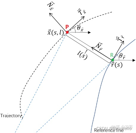
第二步是基于车当前所在的点（x，y），找到参考线上的最近匹配点，为什么要这样做？ 因为参考线是车要循迹的线，车都是在不断向参考线修正的，直到此时和参考线完全重合就是最优的状态。

1. 这一步的思路是，遍历参考线reference_line，找到距离车🚗当前点最近的点，没错就是穷举遍历（相信c++的计算速度😄）。
2. 找到最近点后，不是直接把这个点当成匹配点，而是基于参考线上的该点往前后各找一个点，把这两个点连接成向量，方向向前。
3. 然后把车当前的点（下图P）投影到这个向量上，这个投影点才是第二步要找的匹配点。

  PathPoint matched_point =PathMatcher::MatchToPath(*ptr_reference_line, planning_init_point.path_point().x(),
      planning_init_point.path_point().y());//planning_init_point.path_point()当前定位点

• 根据距离找点

PathPoint PathMatcher::MatchToPath(const std::vector<PathPoint>& reference_line,constdouble x,constdouble y){//x、y是当前定位点CHECK_GT(reference_line.size(),0U);auto func_distance_square =[](const PathPoint& point,constdouble x,constdouble y){double dx = point.x()- x;double dy = point.y()- y;return dx * dx + dy * dy;//两点距离平方};double distance_min =func_distance_square(reference_line.front(), x, y);
  std::size_t index_min =0;for(std::size_t i =1; i < reference_line.size();++i){//遍历reference_line，找到距离最小的点的double distance_temp =func_distance_square(reference_line[i], x, y);//计算当前点到reference_line上i点的距离if(distance_temp < distance_min){
      distance_min = distance_temp;//距离
      index_min = i;//点的索引}}//向后找一个点
  std::size_t index_start =(index_min ==0)? index_min : index_min -1;//向前找一个点
  std::size_t index_end =(index_min +1== reference_line.size())? index_min : index_min +1;//目的主要是将当前的定位点投影到距离最短点的前后点的连线上，做预处理if(index_start == index_end){return reference_line[index_start];}//投影操作returnFindProjectionPoint(reference_line[index_start],
                             reference_line[index_end], x, y);}

• 找到点之后算当前定位点在参考线上的投影

PathPoint PathMatcher::FindProjectionPoint(const PathPoint& p0,const PathPoint& p1,constdouble x,constdouble y){//P0A向量double v0x = x - p0.x();double v0y = y - p0.y();//P0P1向量double v1x = p1.x()- p0.x();double v1y = p1.y()- p0.y();double v1_norm = std::sqrt(v1x * v1x + v1y * v1y);double dot = v0x * v1x + v0y * v1y;double delta_s = dot / v1_norm;//P0B长度returnInterpolateUsingLinearApproximation(p0, p1, p0.s()+ delta_s);//计算投影点的具体各项数据}

手绘图：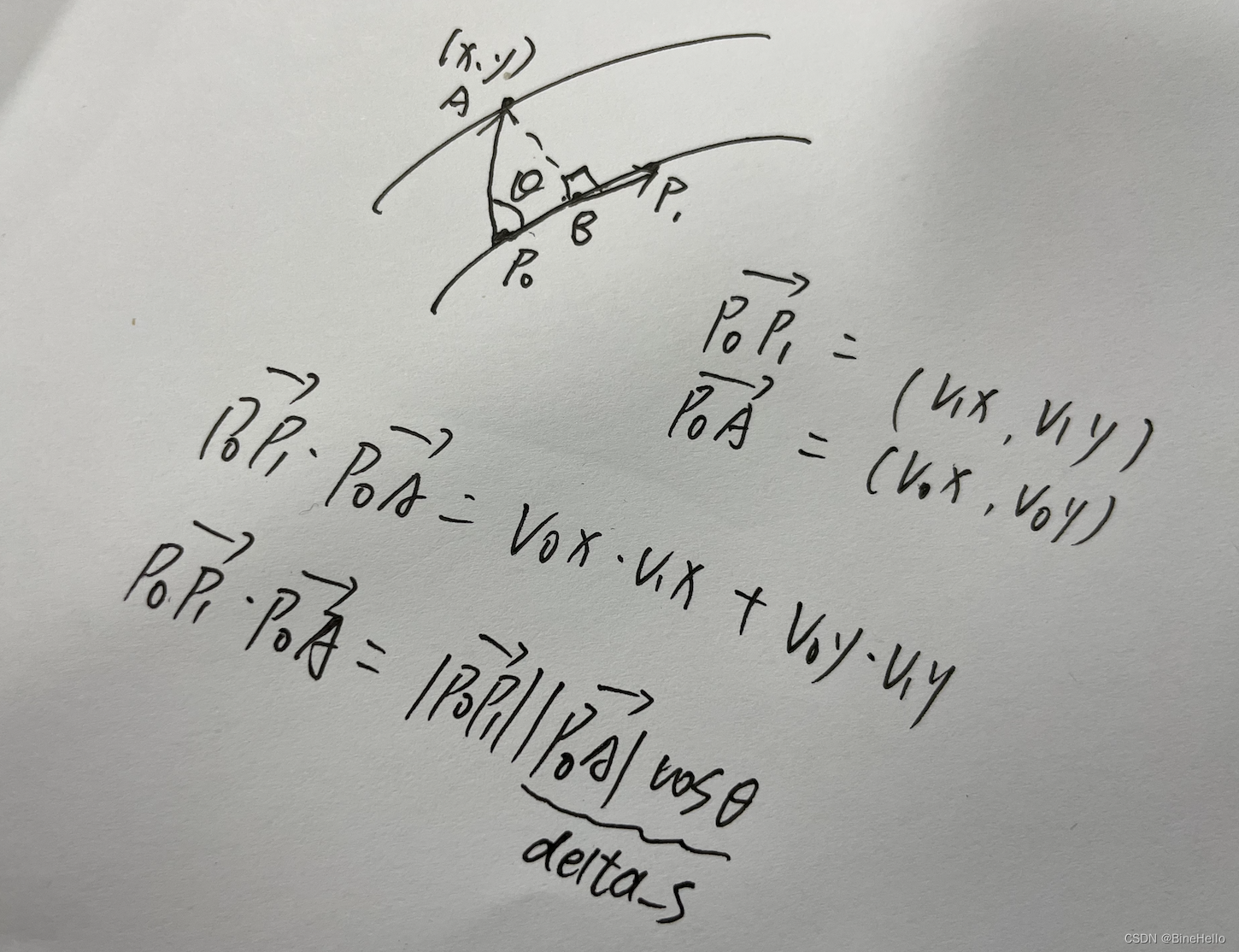

简单理解一下这个图就能看懂代码了。😁😁

• 计算投影点的具体各项数据

为了得到投影点的具体各项数据，主要在上面的两点之间用线性插值（主要根据占比权重来算）,公式做了合并同类项。

PathPoint InterpolateUsingLinearApproximation(const PathPoint &p0,const PathPoint &p1,constdouble s){double s0 = p0.s();double s1 = p1.s();

  PathPoint path_point;double weight =(s - s0)/(s1 - s0);//p0.x()+weight*(p1.x()-p0.x())double x =(1- weight)* p0.x()+ weight * p1.x();double y =(1- weight)* p0.y()+ weight * p1.y();double theta =slerp(p0.theta(), p0.s(), p1.theta(), p1.s(), s);double kappa =(1- weight)* p0.kappa()+ weight * p1.kappa();double dkappa =(1- weight)* p0.dkappa()+ weight * p1.dkappa();double ddkappa =(1- weight)* p0.ddkappa()+ weight * p1.ddkappa();
  path_point.set_x(x);
  path_point.set_y(y);
  path_point.set_theta(theta);
  path_point.set_kappa(kappa);//曲率
  path_point.set_dkappa(dkappa);//曲率求导
  path_point.set_ddkappa(ddkappa);
  path_point.set_s(s);return path_point;}

3. 根据匹配点，计算Frenet坐标系的S-L值

第3步的是计算车当前点P在Frenet坐标系下的坐标，这部分的原理可参考其他博客，主要就是套公式转换一下，为下面在S-T图的生成生成做准备。
在Frenet坐标系下的s就是第一步计算的s，L大小是上面手绘图的

    ∣
   
   
    A
   
   
    B
   
   
    ∣
   
  
  
   |AB|
  
 
∣AB∣，方向和

 
  
   
    
     P
    
    
     0
    
   
   
    
     P
    
    
     1
    
   
  
  
   P_{0}P_{1}
  
 
P0​P1​垂直，指向A。

  std::array<double,3> init_s;
  std::array<double,3> init_d;ComputeInitFrenetState(matched_point, planning_init_point,&init_s,&init_d);auto ptr_prediction_querier = std::make_shared<PredictionQuerier>(
      frame->obstacles(), ptr_reference_line);

补充说明一下，Frenet坐标系就是S-L坐标系，Frenet坐标系下的参数主要还是s，l，s就是累积距离，l就是后面提到的d，类似横向距离。

4. parse the decision and get the planning target

该部分总体代码：

// 加入感知信息时，里面涉及多个函数，具体包括障碍物筛选，去掉与车辆未来轨迹不发生冲突的障碍物，设置动态障碍物。auto ptr_path_time_graph = std::make_shared<PathTimeGraph>(
      ptr_prediction_querier->GetObstacles(),*ptr_reference_line,
      reference_line_info, init_s[0]起始点,
      init_s[0]+ FLAGS_speed_lon_decision_horizon=200,0.0,
      FLAGS_trajectory_time_length=8s, init_d);double speed_limit =
      reference_line_info->reference_line().GetSpeedLimitFromS(init_s[0]);
  reference_line_info->SetLatticeCruiseSpeed(speed_limit);//限制巡航速度

  PlanningTarget planning_target = reference_line_info->planning_target();

这部分是计算障碍物的S-T图，这里的S是frenet下的s，t是时间。这部分接收感知那边传来的障碍物信息，计算障碍物在frenet坐标系下的最大值和最小值，代码如下：

SLBoundary PathTimeGraph::ComputeObstacleBoundary(const std::vector<common::math::Vec2d>& vertices,const std::vector<PathPoint>& discretized_ref_points)const{doublestart_s(std::numeric_limits<double>::max());doubleend_s(std::numeric_limits<double>::lowest());doublestart_l(std::numeric_limits<double>::max());doubleend_l(std::numeric_limits<double>::lowest());for(constauto& point : vertices){//转frenet坐标auto sl_point =PathMatcher::GetPathFrenetCoordinate(discretized_ref_points,
                                                         point.x(), point.y());//计算障碍物在s-l坐标系下的最大值最小值
    start_s = std::fmin(start_s, sl_point.first);
    end_s = std::fmax(end_s, sl_point.first);
    start_l = std::fmin(start_l, sl_point.second);
    end_l = std::fmax(end_l, sl_point.second);}

  SLBoundary sl_boundary;//下图障碍物的显示
  sl_boundary.set_start_s(start_s);
  sl_boundary.set_end_s(end_s);
  sl_boundary.set_start_l(start_l);
  sl_boundary.set_end_l(end_l);return sl_boundary;}

像上图描述的，就是将障碍物投影到frenet坐标系下，和车的预瞄轨迹点是否有交集（apollo 的预瞄距离是200米），没有交集的就不需要考虑。

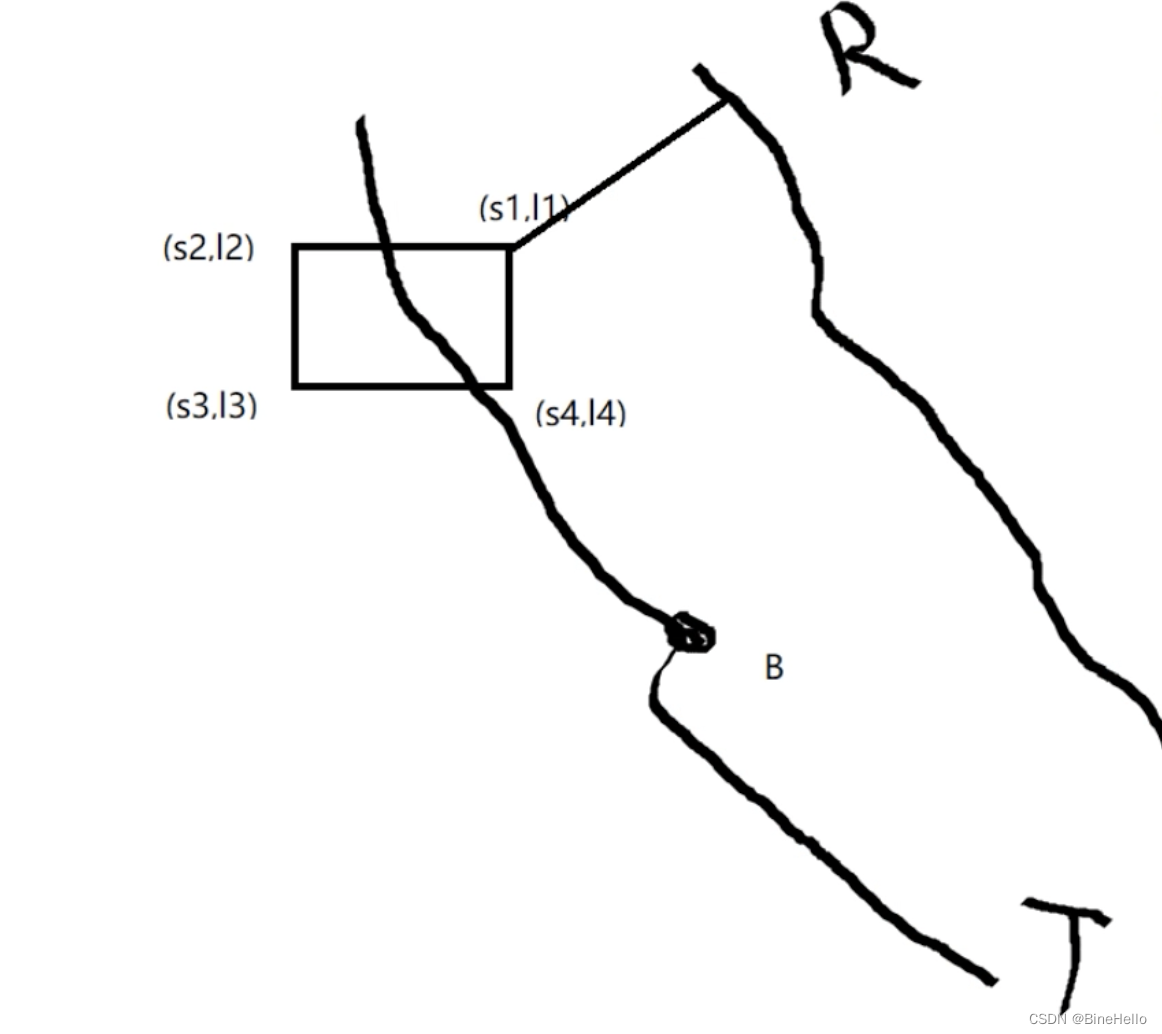
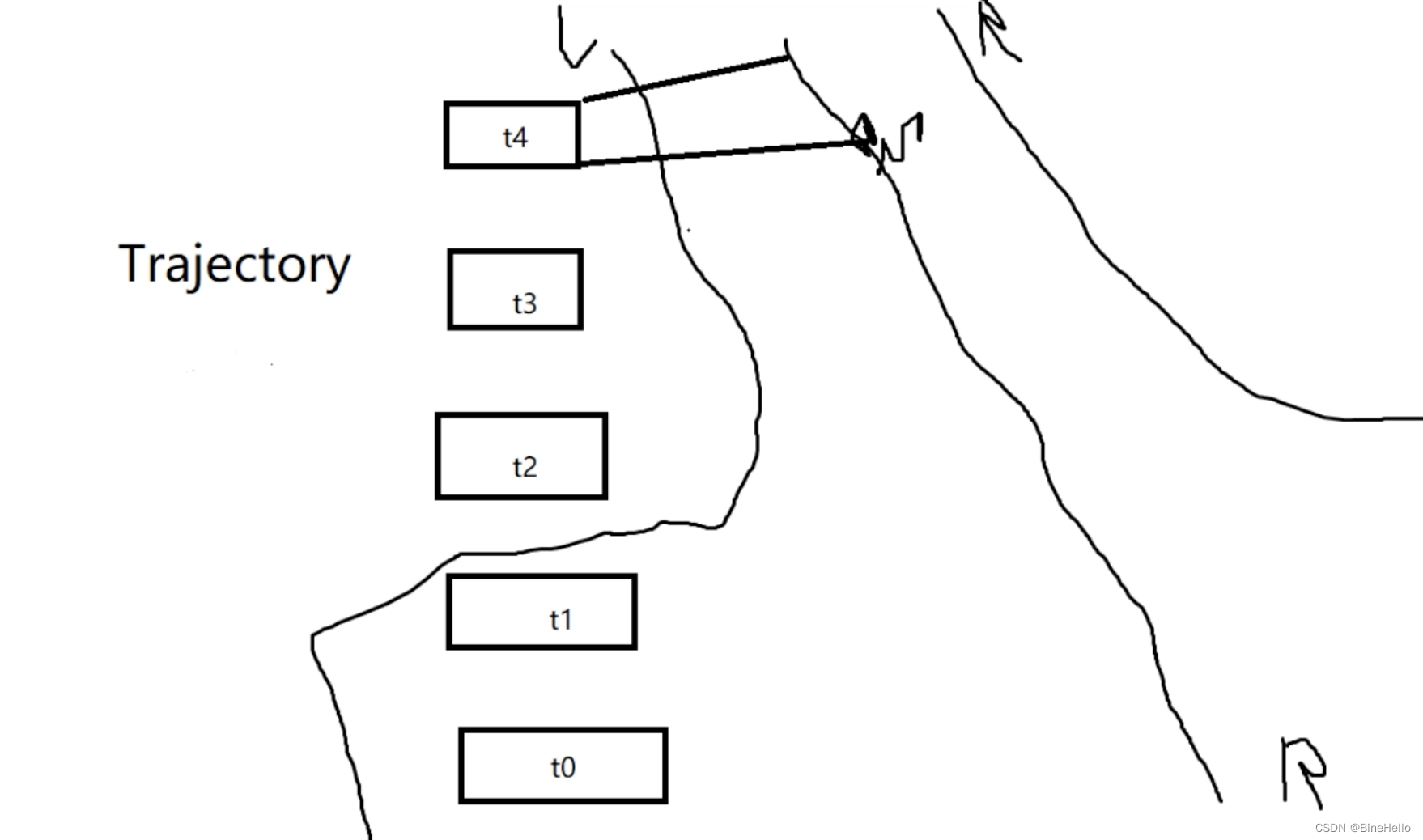
动态障碍物的思路大概一样，动态障碍物可以看作多个静态障碍物，如下图，主要都是投影到frenet坐标系下，为下一步在S-T图上表达障碍物，以及在S- T图上做撒点采样，生成轨迹做铺垫。

解析一下这个图，中间是🚗轨迹，左右分别是车道边界，t0，t1在车道线内则考虑，其他时刻不考虑，其实详细思路更加复杂😭。

到这里，我们就能够得到障碍物的距S-T图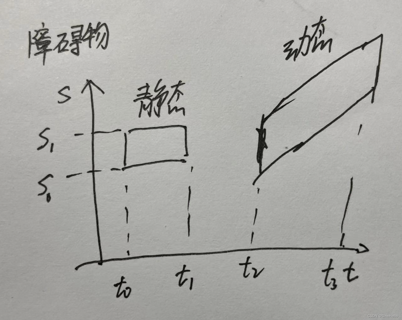

5. 生成横纵向采样路径

这步是关键，前面的Frenet坐标系和障碍物的S-T图可以说都是为了后面生成轨迹做铺垫的。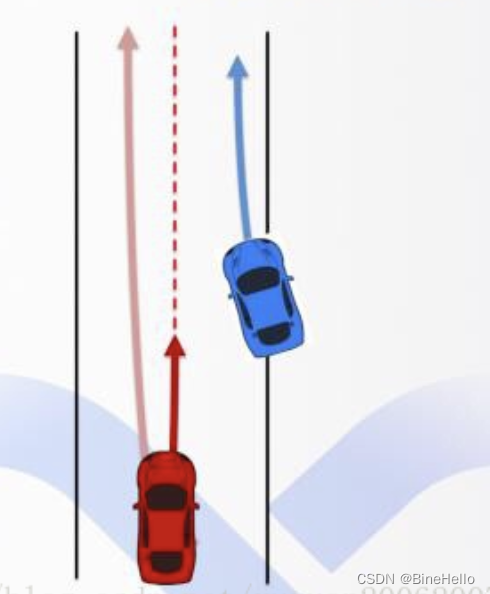

对于上图，有些司机会按照右图中浅红色的轨迹，选择绕开蓝色的障碍车。另外有一些司机开车相对保守，会沿着右图中深红色较短的轨迹做一个减速，给蓝色障碍车让路。

既然对于同一个场景，人类司机会有多种处理方法，那么Lattice规划算法的第一步就是采样足够多的轨迹，提供尽可能多的选择。

如何进行横纵向采样呢？

• 横向采样

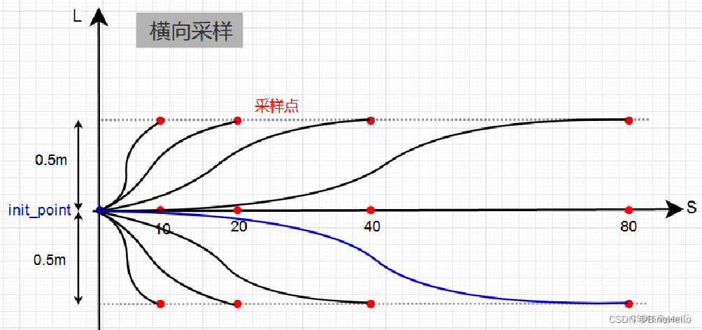
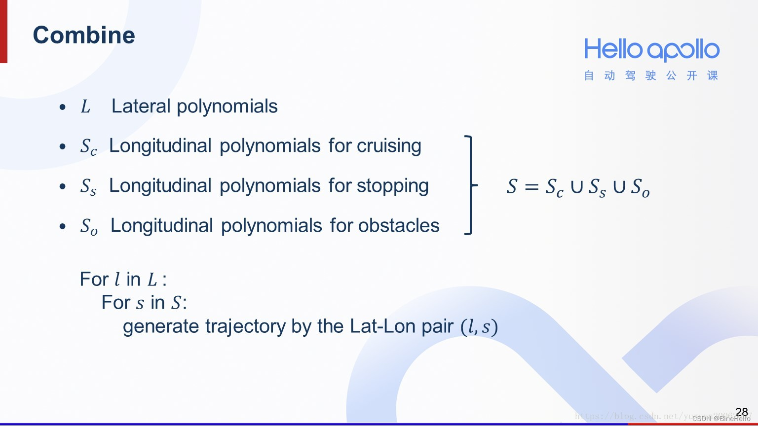
横向轨迹的采样需要涵盖多种横向运动状态。现在Apollo的代码中设计了三个末状态横向偏移量，**-0.5，0.0和0.5，以及四个到达这些横向偏移量的纵向位移，分别为10，20，40，80**。用两层循环遍历各种组合，再通过多项式拟合，即可获得一系列的横向轨迹。

• 纵向采样纵向轨迹采样需要考虑巡航、跟车或超车、停车这三种状态。也就是说3种情况下都要生成轨迹，后面再进行评估选择cost小的。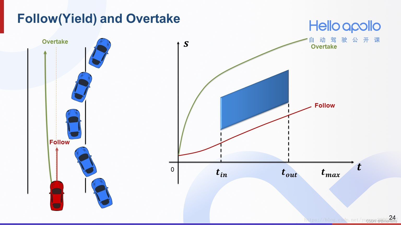有了S-T图的概念，观察左图中的两条规划轨迹。红色的是一条跟车轨迹，绿色的是超车轨迹。这两条轨迹反映在S-T图中，就如右图所示。红色的跟车轨迹在蓝色阴影区域下方，绿色的超车轨迹在蓝色阴影区域上方。如果有多个障碍物，就对这些障碍物分别采样超车和跟车所对应的末状态。 总结下来就是遍历所有和车道有关联的障碍物，对他们分别采样超车和跟车的末状态，然后用多项式拟合即可获得一系列纵向轨迹。多项式拟合如何生成多项式轨迹？可以看一下下面这篇blog。

无人车-运动规划-高阶多项式曲线方程求解

上图是将所有的轨迹整合，交给下一步来评估。

Lattice Planner会根据起点和终点的状态，在位置空间和时间上同时进行撒点。撒点的起始状态和终止状态各有6个参数，包括了3个横向参数，即横向位置、横向位置的导数和导数的导数；3个纵向参数，即纵向位置、纵向位置的一阶导数也就是速度、纵向位置的二阶导数（也就是加速度）。

起点的参数是车辆当时真实的状态，终点状态则是撒点枚举的各个情况。在确定了终点和起点状态以后，再通过五阶或者四阶的多项式连接起始状态和终止状态，从而得到规划的横向和纵向轨迹。

6. 轨迹cost值计算，进行碰撞检测

有了轨迹的cost以后，就是一个循环检测的过程。在这个过程中，每次会先挑选出cost最低的轨迹，对其进行物理限制检测和碰撞检测。如果挑出来的轨迹不能同时通过这两个检测，就将其筛除，考察下一条cost最低的轨迹。

  TrajectoryEvaluator trajectory_evaluator(
      init_s, planning_target, lon_trajectory1d_bundle, lat_trajectory1d_bundle,
      ptr_path_time_graph, ptr_reference_line);// Get instance of collision checker and constraint checker
  CollisionChecker collision_checker(frame->obstacles(), init_s[0], init_d[0],*ptr_reference_line, reference_line_info,
                                     ptr_path_time_graph);

7. 优先选择cost最小的轨迹且不碰撞的轨迹

获得采用轨迹之后，接着需要进行目标轨迹的曲率检查和碰撞检测，目的是为了使目标采样轨迹满足车辆的运动学控制要求和无碰撞要求，这样就形成了安全可靠的轨迹簇。这些轨迹簇都可以满足车辆的控制要求，但并不是最优的，因此需要从轨迹簇中选出一组最优的运行轨迹。这时就需要引入轨迹评价函数，用来对候选轨迹进行打分。

轨迹评价函数主要为了使得目标轨迹尽量靠近静态参考线轨迹运行，同时，速度尽量不发生大突变，满足舒适性要求，且尽量远离障碍物。因此最后轨迹评价函数可以通过如下伪代码描述：

traj_cost = k_lat * cost_lat + k_lon * cost_lon + k_obs * obs_cost;

上式中：
k_lat : 表示纵向误差代价权重
cost_lat： 表示纵向误差，综合考虑纵向速度误差，时间误差及加加速度的影响。
k_lon : 表示横向误差代价权重
cost_lon： 表示横向向误差，综合考虑了横向加速度误差及横向偏移误差的影响。
k_obs : 表示障碍物代价权重
obs_cost： 表示障碍物距离损失。
最后选择出代价值最好的一条轨迹输入到控制器，用于控制器的跟踪控制。

while(trajectory_evaluator.has_more_trajectory_pairs()){double trajectory_pair_cost =
        trajectory_evaluator.top_trajectory_pair_cost();auto trajectory_pair = trajectory_evaluator.next_top_trajectory_pair();// combine two 1d trajectories to one 2d trajectoryauto combined_trajectory =TrajectoryCombiner::Combine(*ptr_reference_line,*trajectory_pair.first,*trajectory_pair.second,
        planning_init_point.relative_time());// check longitudinal and lateral acceleration// considering trajectory curvaturesauto result =ConstraintChecker::ValidTrajectory(combined_trajectory);if(result != ConstraintChecker::Result::VALID){++combined_constraint_failure_count;switch(result){case ConstraintChecker::Result::LON_VELOCITY_OUT_OF_BOUND:
          lon_vel_failure_count +=1;break;case ConstraintChecker::Result::LON_ACCELERATION_OUT_OF_BOUND:
          lon_acc_failure_count +=1;break;case ConstraintChecker::Result::LON_JERK_OUT_OF_BOUND:
          lon_jerk_failure_count +=1;break;case ConstraintChecker::Result::CURVATURE_OUT_OF_BOUND:
          curvature_failure_count +=1;break;case ConstraintChecker::Result::LAT_ACCELERATION_OUT_OF_BOUND:
          lat_acc_failure_count +=1;break;case ConstraintChecker::Result::LAT_JERK_OUT_OF_BOUND:
          lat_jerk_failure_count +=1;break;case ConstraintChecker::Result::VALID:default:// Intentional emptybreak;}continue;}// check collision with other obstaclesif(collision_checker.InCollision(combined_trajectory)){++collision_failure_count;continue;}// put combine trajectory into debug dataconstauto& combined_trajectory_points = combined_trajectory;
    num_lattice_traj +=1;
    reference_line_info->SetTrajectory(combined_trajectory);
    reference_line_info->SetCost(reference_line_info->PriorityCost()+
                                 trajectory_pair_cost);
    reference_line_info->SetDrivable(true);// Print the chosen end condition and start condition
    ADEBUG <<"Starting Lon. State: s = "<< init_s[0]<<" ds = "<< init_s[1]<<" dds = "<< init_s[2];// castauto lattice_traj_ptr =
        std::dynamic_pointer_cast<LatticeTrajectory1d>(trajectory_pair.first);if(!lattice_traj_ptr){
      ADEBUG <<"Dynamically casting trajectory1d ptr. failed.";}}}

总结

总体讲清楚了算法的过程，但是代码层面涉及太多，后面还得慢慢深入，特别是采样的过程的代码得再解析。

参考：
Baidu Apollo 6.2 Lattice Planner规划算法
Apollo星火计划学习笔记——第七讲自动驾驶规划技术原理1
Lattice算法之六轨迹评估