2023美国大学生数学建模竞赛E题光污染完整数据集和求解代码分享

2023美国大学生数学建模竞赛E题进度：目前已完成2023美赛E题光污染数据集和相关代码的分析。数据集总共1.2GB

​

​

​

​

数据集收集

GeoNames 地理数据集

GeoNames地理数据库涵盖所有国家，包含超过一千一百万个可供免费下载的地名。该数据集包含一些关键信息，例如大陆、面积（km^ 2）和人口。

全球各国的经纬度数据集

Google Developers，其中包含每个国家/地区的经纬度数据。这为该国确定了一个合理的中心。

协调一致的全球夜间灯光（1992 - 2018）数据集

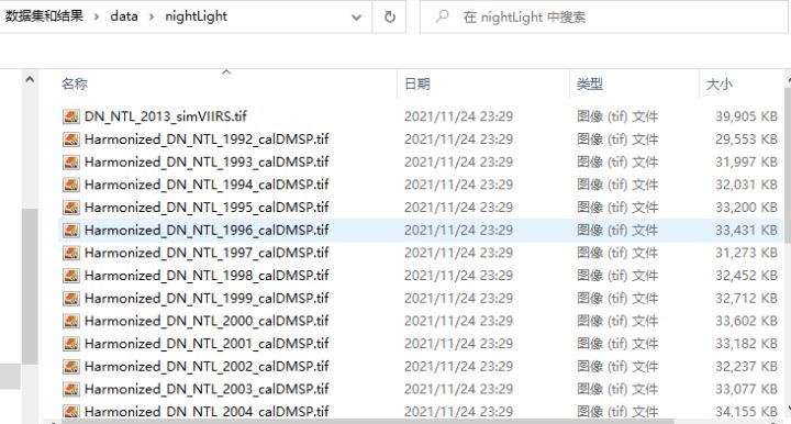
这个数据集特别大，包含近 200 亿个数据点（特别是20322960028），因此必须以块的形式获取这些数据。所有数据都可以从 zip 文件中下载，如下所示。

1. 下载 zip 文件
2. 创建一个与此笔记本相关的目录，名为data/nightLight
3. 将 zip 文件中的所有内容解压缩到nightLight步骤 2 中创建的目录中。
4. 删除 zip 文件，以节省磁盘空间。

fig, (axim, axhist) = plt.subplots(1, 2, figsize=(40, 10), gridspec_kw={'width_ratios': [3, 1]})
rf = rs.open("data/nightLight/DN_NTL_2013_simVIIRS.tif", "r")
show(rf, ax=axim, cmap="inferno")
show_hist(rf, ax=axhist)
axim.set(xlabel="Longitude", ylabel="Latitude", title="Image of 2013 VIIRS Data")
axhist.set_title("Color Historgram of 2013 VIIRS Data")
del rf

​

NASA 的 EaN Blue Marble 2016 数据集

至少 25 年来，地球夜间的卫星图像（通常被称为“夜灯”）一直是公众的好奇心和基础研究的工具。他们提供了一幅广阔而美丽的图画，展示了人类如何塑造地球并照亮黑暗。这些地图每十年左右制作一次，催生了数百种流行文化用途和数十个经济、社会科学和环境研究项目。

这些图像显示了 2016 年观测到的地球夜间灯光。这些数据经过新的合成技术重新处理，该技术选择了每个陆地上每个月最好的无云夜晚。

这些图像以 JPEG 和 GeoTIFF 格式提供，具有三种不同的分辨率：0.1 度 ( 3600x1800)、3 公里 ( 13500x6750) 和 500 米 ( 86400x43200)。500 米的全球地图根据网格化方案分为多个图块 (21600x21600)。

全球夜间数据集

Globe At Night 根据特定位置收集数据，在这种情况下，包含一个名为的列，LimitingMag该列可以与该地区的光污染标准相关。

以下命令展示了一种以编程方式下载数据集的方法，同时还删除了不必要的数据集。

gan_url = "https://www.globeatnight.org/"
files = [gan_url + i["href"] for i in BeautifulSoup(requests.get(gan_url+"maps.php").content, "lxml").findAll(href=re.compile("\.csv$"))]
gan = []
for file in files:
    filename = "data/gan/"+file.split("/")[-1]
    print(file, "==>", filename)
    file = BytesIO(requests.get(file, allow_redirects=True).content)
    data = pd.read_csv(file, error_bad_lines=False)[["Latitude", "Longitude", "LocalDate", "LocalTime", "UTDate", "UTTime", "LimitingMag", "Country"]]
    data = data[data.LimitingMag > 0]
    data.LocalTime = pd.to_datetime(data.apply(lambda row: row["LocalDate"] + " " + row["LocalTime"], axis=1), format='%Y-%m-%d %H:%M')
    data.UTTime = pd.to_datetime(data.apply(lambda row: row["UTDate"] + " " + row["UTTime"], axis=1), format='%Y-%m-%d %H:%M')
    data.loc[:, "Year"] = int(filename[-8:-4])
    data = data[["Latitude", "Longitude", "LocalTime", "UTTime", "LimitingMag", "Country", "Year"]]
    data.to_csv(filename)
    gan.append(data)

gan = pd.concat(gan, ignore_index=True)
gan.to_csv("data/gan/GaN.csv", index=False)

读取数据集

gan = pd.read_csv("data/gan/GaN.csv").sort_values(["Year", "Country"], ignore_index=True)
gan.Country = gan.Country.str.replace("United States.*", "United States").str.replace("Republic of the Union of Myanmar", "Myanmar").replace("Republic of the Congo", "Congo Republic").replace('Myanmar (Burma)', "Myanmar").replace("Czechia", "Czech Republic").replace("Republic of Kosovo", "Kosovo").replace("Brunei Darussalam", "Brunei").replace("Democratic Republic of the Congo", "DR Congo").replace("The Bahamas", "Bahamas").replace('Macedonia (FYROM)', "North Macedonia").replace("Reunion", "Réunion").replace('Virgin Islands', 'U.S. Virgin Islands').replace('St Vincent and the Grenadines', 'St Vincent and Grenadines').replace('Kingdom of Norway', "Norway").replace('The Netherlands', 'Netherlands')

gan_countries = set(gan.Country.unique())
geolatlong_countries = set(geocountries_latlong.Country.unique())
print(gan_countries - geolatlong_countries)
print(geolatlong_countries - gan_countries)
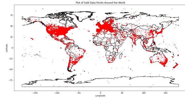
base = countries.plot(color='white', edgecolor='black')
gan[["geometry"]].plot(ax=base, marker='o', color='red', markersize=2)
_ = (base.set_xlabel("Longitude"), base.set_ylabel("Latitude"), base.set_title("Plot of GaN Data Points Around the World"))

​

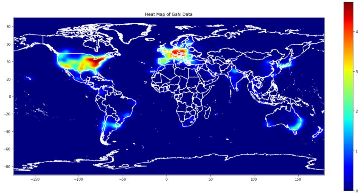
绘制热图

heatmap, xedges, yedges = np.histogram2d(gan.Latitude, gan.Longitude, bins=250)

logheatmap = np.log(heatmap)
logheatmap[np.isneginf(logheatmap)] = 0
logheatmap = sp.ndimage.filters.gaussian_filter(logheatmap, 2, mode='nearest')

plt.figure(figsize=(20, 10))

plt.imshow(logheatmap, cmap="jet", extent=[yedges[0], yedges[-1], xedges[-1], xedges[0]])
plt.colorbar()

ax = plt.gca()
ax.invert_yaxis()
ax.set_xlim(-175,180)

countries.boundary.plot(edgecolor='white', ax=ax)
_ = ax.set_title("Heat Map of GaN Data")

​

光污染分析

代码如下：

​

​

在这里，我们使用以下两种不同的算法来大致了解光污染：

pivotNightLight = nightLightMean.pivot("Country", "Year", "Average Light Pollution").sort_values(2018).rename(columns="nightLight{}".format) pivotNightLight

​

defsummary(data, xloc, yloc):
    x, y = data.Year, data["Average Light Pollution"]
    m, c, r, p, stderr = stats.linregress(x=x, y=y)
    mspe = mean_squared_error(y, m*x + c)
    sns.regplot(x=x, y=y)
    plt.text(xloc, yloc, f"$y = {m} x + {c}$\nCorrelation, $r = {r}$\nConfidence, $p = {p}$\n$R^2 = {r**2}$\n$MSPE = {mspe}$")

yr_based = pivotNightLight.rename(columns=lambda yrstr: int(yrstr[-4:])).mean(axis=0).reset_index().rename(columns={0: "Average Light Pollution"})
summary(data=yr_based, xloc=2005, yloc=6)
plt.title("Regression plots of Double Average Light Pollution, $\mu_1$ per Year")

​

nightLightByQuan = nightLight[nightLight.Quantity.isin(["mean", "count"])].reset_index().set_index(["Quantity", "Year"])
fitted_mean_by_yr = ((nightLightByQuan.loc["mean"] * nightLightByQuan.loc["count"]).sum(axis=1) / nightLightByQuan.loc["count"].sum(axis=1)).reset_index().rename(columns={0:"Average Light Pollution"})
summary(fitted_mean_by_yr, 2004, 2.5)
summary(fitted_mean_by_yr[fitted_mean_by_yr.Year.isin(range(1992, 2014))], 2004, 0.6)
sns.lineplot(data=fitted_mean_by_yr, x="Year", y="Average Light Pollution").axvspan(xmin=2013.5, xmax=2018.5, color="r", alpha=0.2)
plt.title("Regression plots of Overall Weighted Average Light Pollution, $\mu_2$ per Year")

​

nightLightHighLow = nightLight.reset_index().set_index(["Quantity", "Year"]).loc["mean"].T.stack().reset_index().rename(columns={"level_0": "Country", 0: "Value"}).groupby("Country").Value.agg(["max", "min"])
nightLightHighLow = (nightLightHighLow["max"] - nightLightHighLow["min"]).sort_values(ascending=False).iloc[:5]
predict(nightLightHighLow)

​

defnightLightFilter(slice):
    return nightLight.reset_index().set_index(["Year", "Quantity"]).T.sort_values((2018, "mean"), ascending=False).iloc[slice].T.stack().reset_index().set_index(["Quantity", "Year"]).loc[["mean", "min", "max", "median", "mode"]].reset_index().rename(columns={"level_2":"Country", 0: "Value"})

nightLightMax = nightLightFilter(slice(0, 5))
for alg in [sns.lineplot, sns.regplot, sns.residplot]:
    sns.FacetGrid(nightLightMax, col="Quantity", row="Country").map(alg, "Year", "Value")

​

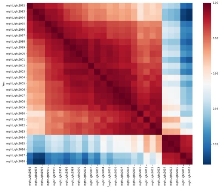
fig, ax = plt.subplots(1, figsize=(15, 12))
sns.heatmap(pivotNightLight.corr().dropna(how="all", axis=0).dropna(how="all", axis=1), cmap="RdBu_r", ax=ax)

​

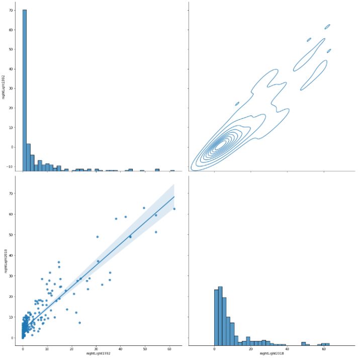
sns.PairGrid(pivotNightLight[["nightLight1992", "nightLight2018"]], height=8).map_diag(sns.histplot).map_lower(sns.regplot).map_upper(sns.kdeplot)

​

​数据集和代码地址

2023美国大学生数学建模竞赛E题光污染数据集