人工智能|机器学习——Canopy聚类算法（密度聚类）

1.简介

Canopy聚类算法是一个将对象分组到类的简单、快速、精确地方法。每个对象用多维特征空间里的一个点来表示。这个算法使用一个快速近似距离度量和两个距离阈值T1 > T2 处理。

Canopy聚类很少单独使用， 一般是作为k-means前不知道要指定k为何值的时候，用Canopy聚类来判断k的取值

2.算法步骤

输入：所有点的集合D， 超参数：T1 , T2 , 且 T1 > T2

输出：聚类好的集合

注意

• 当T1过大时，会使许多点属于多个Canopy，可能会造成各个簇的中心点间距离较近，各簇间区别不明显；
• 当T2过大时，增加强标记数据点的数量，会减少簇个个数；
• T2过小，会增加簇的个数，同时增加计算时间；

一幅图说明算法：

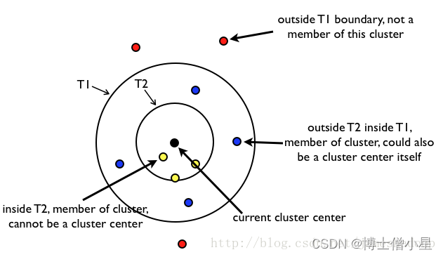
内圈的一定属于该类， 外圈的一定不属于该类， 中间层的可能属于别的类（因为不止一个聚类中心， 他可能属于别的类的内圈）；

3.python实现

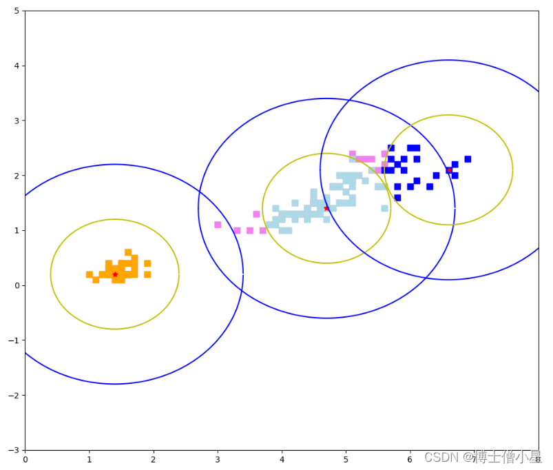
对iris数据集做Canopy聚类， 半径分别设置为1和2

#%% Canopy聚类
import pandas as pd
from sklearn.cluster import KMeans
import matplotlib.pyplot as plt
import numpy as np
import copy
class Solution(object):
    def Canopy(self, x, t1, t2):
        '''
        
    
        Parameters
        ----------
        x : array
            数据集.
        t1 : float
            外圈半径.
        t2 : float
            内圈半径.
    
        Returns
        -------
        result: list.
            聚好类的数据集
        '''
        if t1 < t2:
            return print("t1 应该大于 t2")
        x = copy.deepcopy(x)
        result = []  # 用于存放最终结果
        index = np.zeros((len(x),))   # 用于标记外圈外的点 1表示强标记， 2表示弱标记
        while (index == np.zeros((len(x),))).any():
            alist = []  # 用于存放某一类的数据集
            choice_index = None
            for i, j in enumerate(index):
                if j == 0:
                    choice_index = i
                    break
            C = copy.deepcopy(x[choice_index])
            alist.append(C)
            x[choice_index] = np.zeros((1, len(x[0])))
            index[choice_index] = 1
            for i,a in enumerate(x):
                if index[i] != 1:
                    distant = (((a-C)**2).sum())**(1/2)
                    if distant <= t2:  # 打上强标记
                        alist.append(copy.deepcopy(x[i]))
                        x[i] = np.zeros((1, len(x[0])))
                        index[i] = 1
                    elif distant <= t1:
                        index[i] = 2
            result.append(alist)
        return result
def pint(r, x, y, c):
    # 点的横坐标为a
    a = np.arange(x-r,x+r,0.0001)
    # 点的纵坐标为b
    b = np.sqrt(np.power(r,2)-np.power((a-x),2))
    plt.plot(a,y+b,color=c,linestyle='-')
    plt.plot(a,y-b,color=c,linestyle='-')
    plt.scatter(x, y, c='r',marker='*')
if __name__ == '__main__':
    data = pd.read_csv(r'C:/Users/潘登/Documents/python全系列/人工智能/iris.csv')
    X = np.array(data.iloc[:, 2:4])
    Y = data['species']
    result = Solution().Canopy(X, 2, 1)
    x1 = []
    y1 = []
    for i in result[0]:
        x1.append(i[0])
        y1.append(i[1])
    x2 = []
    y2 = []
    for i in result[1]:
        x2.append(i[0])
        y2.append(i[1])
    x3 = []
    y3 = []
    for i in result[2]:
        x3.append(i[0])
        y3.append(i[1])
    plt.figure(figsize=(16,12))
    plt.scatter(X[:,0], X[:,1], s=50, c='violet', marker='s')
    plt.scatter(x1, y1, s=50, c='orange', marker='s')
    plt.scatter(x2, y2, s=50, c='lightblue', marker='s')
    plt.scatter(x3, y3, s=50, c='blue', marker='s')
    pint(2, x1[0], y1[0], 'b')
    pint(1, x1[0], y1[0], 'y')
    pint(2, x2[0], y2[0], 'b')
    pint(1, x2[0], y2[0], 'y')
    pint(2, x3[0], y3[0], 'b')
    pint(1, x3[0], y3[0], 'y')
    plt.xlim([0, 8])
    plt.ylim([-3, 5])
    plt.show()

+结果如下：