​Kaggle M5 Forecasting:传统预测方法与机器学习预测方法对比

本文使用的数据集来自 kaggle：M5 Forecasting — Accuracy。该数据集包含有 California、Texas、Wisconsin 三个州的产品类别、部门、仓储信息等。基于这些数据，需要预测接下来 28 天的每日销售量。

本文代码 github见最后部分

涉及到的方法有：

• 单指数平滑法
• 双指数平滑法
• 三指数平滑法
• ARIMA
• SARIMA
• SARIMAX
• Light Gradient Boosting
• Random Forest
• Linear Regression

---

为了使用上述方法，首先导入相应的包/库：

importtime
importwarnings
importnumpyasnp
importpandasaspd
importseabornassns
importlightgbmaslgb
fromitertoolsimportcycle
fromsklearn.svmimportSVR
importstatsmodels.apiassm
frompmdarimaimportauto_arima
importmatplotlib.pyplotasplt
fromdatetimeimportdatetime, timedelta
fromsklearn.metricsimportmean_squared_error
fromsklearn.linear_modelimportLinearRegression
fromsklearn.ensembleimportRandomForestRegressor
fromstatsmodels.graphics.tsaplotsimportplot_acf
fromstatsmodels.tsa.holtwintersimportSimpleExpSmoothing, ExponentialSmoothing

%matplotlibinline
plt.style.use('bmh')
sns.set_style("whitegrid")
plt.rc('xtick', labelsize=15)
plt.rc('ytick', labelsize=15)
warnings.filterwarnings("ignore")
pd.set_option('max_colwidth', 100)
pd.set_option('display.max_rows', 500)
pd.set_option('display.max_columns', 500)
color_pal = plt.rcParams['axes.prop_cycle'].by_key()['color']
color_cycle = cycle(plt.rcParams['axes.prop_cycle'].by_key()['color'])

然后导入数据集：

data = pd.read_csv('data_for_tsa.csv')
data['date'] = pd.to_datetime(data['date'])
data.head()

数据集前五行数据

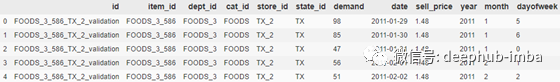
数据集包含了 2011-01-29 到 2016-05-22 期间的 1941 天的数据。其中最后 28 天作为测试集。

预测目标是

demand

，即：当日的产品销售量。

---

接下来进行数据集划分

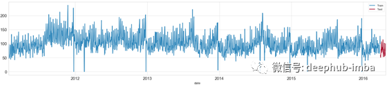
测试集包含了 2016-03-27 到 2016-04-24 期间的 28 天的数据。2016-03-27 之前的其他数据则作为训练数据。

train = data[data['date'] <= '2016-03-27']
test = data[(data['date'] >'2016-03-27') & (data['date'] <= '2016-04-24')]

fig, ax = plt.subplots(figsize=(25,5))
train.plot(x='date',y='demand',label='Train',ax=ax)
test.plot(x='date',y='demand',label='Test',ax=ax);

时间序列数据

---

为了便于对比所有方法的准确性，建立一个命名为

predictions

的 dataframe，将每个方法设为其中的一行。建立一个命名为

stats

的 dataframe，用于存储每个方法的性能表现和计算时间。

predictions = pd.DataFrame()
predictions['date'] = test['date']
stats = pd.DataFrame(columns=['Model Name','Execution Time','RMSE'])

---

训练及评价模型

单指数平滑方法

通过调用

SimpleExpSmoothing

包，可以使用 EWMA, Exponentially Weighted Moving Average方法——一种单指数平滑方法。

使用 EWMA 方法，我们首先需要定义

span

变量——数据集的季节周期。

fig, ax = plt.subplots(figsize=(15, 3))
plot_acf(data['demand'].tolist(), lags=60, ax=ax);

自相关图

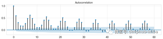
查看数据的自相关图可知，每隔七个数据，达到一个峰值，也就意味着任一数据与之前的第七个时间数据具有较高的相关性。所以这里将

span

设为 7。

具体地，通过以下代码实现单指数平滑方法预测：

t0 = time.time()
model_name='Simple Exponential Smoothing'
span = 7
alpha = 2/(span+1)
#train
simpleExpSmooth_model = SimpleExpSmoothing(train['demand']).fit(smoothing_level=alpha,optimized=False)
t1 = time.time()-t0
#predict
predictions[model_name] = simpleExpSmooth_model.forecast(28).values
#visualize
fig, ax = plt.subplots(figsize=(25,4))
train[-28:].plot(x='date',y='demand',label='Train',ax=ax)
test.plot(x='date',y='demand',label='Test',ax=ax);
predictions.plot(x='date',y=model_name,label=model_name,ax=ax);
#evaluate
score = np.sqrt(mean_squared_error(predictions[model_name].values, test['demand']))
print('RMSE for {}: {:.4f}'.format(model_name,score))

stats = stats.append({'Model Name':model_name, 'Execution Time':t1, 'RMSE':score},ignore_index=True)

单指数平滑方法预测结果

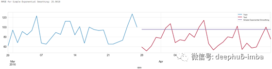
上述代码实现了对于数据的学习，通过

forcast(x),x=28

，预测了接下来 28 天的数据。并且通过均方根误差衡量误差。

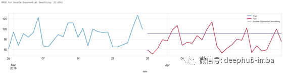
双指数平滑方法

单指数平滑方法只使用了一个平滑系数 ，而双指数平滑方法则引入了第二个平滑系数 ，以反映数据的趋势。使用双指数平滑方法，我们需要定义

seasonal_periods

。

具体代码如下：

t0 = time.time()
model_name='Double Exponential Smoothing'
#train
doubleExpSmooth_model = ExponentialSmoothing(train['demand'],trend='add',seasonal_periods=7).fit()
t1 = time.time()-t0
#predict
predictions[model_name] = doubleExpSmooth_model.forecast(28).values
#visualize
fig, ax = plt.subplots(figsize=(25,4))
train[-28:].plot(x='date',y='demand',label='Train',ax=ax)
test.plot(x='date',y='demand',label='Test',ax=ax);
predictions.plot(x='date',y=model_name,label=model_name,ax=ax);
#evaluate
score = np.sqrt(mean_squared_error(predictions[model_name].values, test['demand']))
print('RMSE for {}: {:.4f}'.format(model_name,score))

stats = stats.append({'Model Name':model_name, 'Execution Time':t1, 'RMSE':score},ignore_index=True)

双指数平滑方法预测结果

三指数平滑方法

三指数平滑方法进一步引入了系数以反映数据的趋势及季节性变化。

具体代码如下：

t0 = time.time()
model_name='Triple Exponential Smoothing'
#train
tripleExpSmooth_model = ExponentialSmoothing(train['demand'],trend='add',seasonal='add',seasonal_periods=7).fit()
t1 = time.time()-t0
#predict
predictions[model_name] = tripleExpSmooth_model.forecast(28).values
#visualize
fig, ax = plt.subplots(figsize=(25,4))
train[-28:].plot(x='date',y='demand',label='Train',ax=ax)
test.plot(x='date',y='demand',label='Test',ax=ax);
predictions.plot(x='date',y=model_name,label=model_name,ax=ax);
#evaluate
score = np.sqrt(mean_squared_error(predictions[model_name].values, test['demand']))
print('RMSE for {}: {:.4f}'.format(model_name,score))

stats = stats.append({'Model Name':model_name, 'Execution Time':t1, 'RMSE':score},ignore_index=True)

三指数平滑方法预测结果

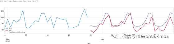
从预测结果可以看出，三指数平滑方法能够学习数据的季节性变化特征。

ARIMA

使用 ARIMA 方法，首先需要确定

p,d,q

三个参数。

• p 是AR项的顺序。
• d 是使时间序列平稳所需的差分次数
• q 是MA项的顺序。

自动确定 ARIMA 所需参数

通过调用

auto_arima

包，可以自动确定 ARIMA 所需的参数。

t0 = time.time()
model_name='ARIMA'
arima_model = auto_arima(train['demand'], start_p=0, start_q=0,
                         max_p=14, max_q=3,
                         seasonal=False,
                         d=None, trace=True,random_state=2020,
                         error_action='ignore',   # we don't want to know if an order does not work
                         suppress_warnings=True,  # we don't want convergence warnings
                         stepwise=True)
arima_model.summary()

auto_arima 的计算结果

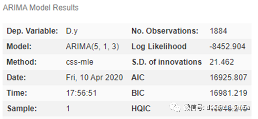
确定了

p,d,q

参数，就可以进行下一步的训练及预测：

#train
arima_model.fit(train['demand'])
t1 = time.time()-t0
#predict
predictions[model_name] = arima_model.predict(n_periods=28)
#visualize
fig, ax = plt.subplots(figsize=(25,4))
train[-28:].plot(x='date',y='demand',label='Train',ax=ax)
test.plot(x='date',y='demand',label='Test',ax=ax);
predictions.plot(x='date',y=model_name,label=model_name,ax=ax);
#evaluate
score = np.sqrt(mean_squared_error(predictions[model_name].values, test['demand']))
print('RMSE for {}: {:.4f}'.format(model_name,score))

stats = stats.append({'Model Name':model_name, 'Execution Time':t1, 'RMSE':score},ignore_index=True)

ARIMA 预测结果

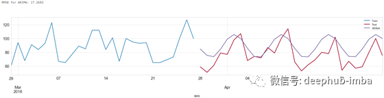
这里使用的简单ARIMA模型不考虑季节性，是一个（5，1，3）模型。这意味着它使用5个滞后来预测当前值。移动窗口的大小等于 1，即滞后预测误差的数量等于1。使时间序列平稳所需的差分次数为 3。

SARIMA

SARIMA 是 ARIMA 的发展，进一步引入了相关参数以使得模型能够反映数据的季节变化特征。

通过

auto_arima

相关代码，将参数设置为

seasonal=True

,

m=7

，自动计算 SARIMA 所需的参数。

t0 = time.time()
model_name='SARIMA'
sarima_model = auto_arima(train['demand'], start_p=0, start_q=0,
                         max_p=14, max_q=3,
                         seasonal=True, m=7,
                         d=None, trace=True,random_state=2020,
                         out_of_sample_size=28,
                         error_action='ignore',   # we don't want to know if an order does not work
                         suppress_warnings=True,  # we don't want convergence warnings
                         stepwise=True)
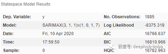
sarima_model.summary()

auto_arima 计算结果

确定了参数后，接下来进行训练及预测：

#train
sarima_model.fit(train['demand'])
t1 = time.time()-t0
#predict
predictions[model_name] = sarima_model.predict(n_periods=28)
#visualize
fig, ax = plt.subplots(figsize=(25,4))
train[-28:].plot(x='date',y='demand',label='Train',ax=ax)
test.plot(x='date',y='demand',label='Test',ax=ax);
predictions.plot(x='date',y=model_name,label=model_name,ax=ax);
#evaluate
score = np.sqrt(mean_squared_error(predictions[model_name].values, test['demand']))
print('RMSE for {}: {:.4f}'.format(model_name,score))

stats = stats.append({'Model Name':model_name, 'Execution Time':t1, 'RMSE':score},ignore_index=True)

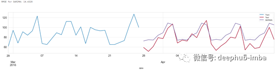
SARIMA 预测结果

SARIMAX

使用前面的方法，我们只能基于前面的历史数据进行预测。在 SARIMAX 中引入外生回归因子（eXogenous regressors），可以实现对时间序列数据以外的数据的分析。

本例中，我们引入

sell_price

数据以辅助更好地预测。

t0 = time.time()
model_name='SARIMAX'
sarimax_model = auto_arima(train['demand'], start_p=0, start_q=0,
                         max_p=14, max_q=3,
                         seasonal=True, m=7,
                         exogenous = train[['sell_price']].values,
                         d=None, trace=True,random_state=2020,
                         out_of_sample_size=28,
                         error_action='ignore',   # we don't want to know if an order does not work
                         suppress_warnings=True,  # we don't want convergence warnings
                         stepwise=True)
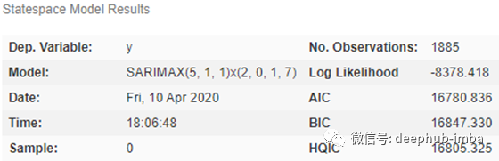
sarimax_model.summary()

auto_arima 计算结果

通过 auto_arima 自动计算了 SARIMAX 方法所需的参数后，可以直接进行训练和预测。

#train
sarimax_model.fit(train['demand'])
t1 = time.time()-t0
#predict
predictions[model_name] = sarimax_model.predict(n_periods=28)
#visualize
fig, ax = plt.subplots(figsize=(25,4))
train[-28:].plot(x='date',y='demand',label='Train',ax=ax)
test.plot(x='date',y='demand',label='Test',ax=ax);
predictions.plot(x='date',y=model_name,label=model_name,ax=ax);
#evaluate
score = np.sqrt(mean_squared_error(predictions[model_name].values, test['demand']))
print('RMSE for {}: {:.4f}'.format(model_name,score))

stats = stats.append({'Model Name':model_name, 'Execution Time':t1, 'RMSE':score},ignore_index=True)

SARIMA 预测结果

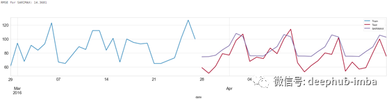
从预测结果可以看出，通过分析额外的数据，有助于减少误差。

机器学习

使用机器学习方法，首先需要特征数据以及指标数据。

在本文中，基于时间序列数据构造特征数据如下：

• 特征数据1：滞后数据。选择 7 天前的 demand 数据作为特征数据。
• 特征数据2：移动平均数据。选择 7 天前至 14 天之前的 demand 移动平均值数据作为特征数据。
• 特征数据3：月销售均值
• 特征数据4：每月销售最大值
• 特征数据5：每月销售最小值
• 特征数据6：每月销售最大值与最小值的差值
• 特征数据7：每周销售均值
• 特征数据8：每周销售最大值
• 特征数据9：每周销售中值

具体代码如下：

deflags_windows(df):
   lags = [7]
   lag_cols = ["lag_{}".format(lag) forlaginlags ]
   forlag, lag_colinzip(lags, lag_cols):
       df[lag_col] = df[["id","demand"]].groupby("id")["demand"].shift(lag)

   wins = [7]
   forwininwins :
       forlag,lag_colinzip(lags, lag_cols):
           df["rmean_{}_{}".format(lag,win)] = df[["id", lag_col]].groupby("id")[lag_col].transform(lambdax : x.rolling(win).mean())  
   returndf

defper_timeframe_stats(df, col):
   #For each item compute its mean and other descriptive statistics for each month and dayofweek in the dataset
   months = df['month'].unique().tolist()
   foryinmonths:
       df.loc[df['month'] == y, col+'_month_mean'] = df.loc[df['month'] == y].groupby(['id'])[col].transform(lambdax: x.mean()).astype("float32")
       df.loc[df['month'] == y, col+'_month_max'] = df.loc[df['month'] == y].groupby(['id'])[col].transform(lambdax: x.max()).astype("float32")
       df.loc[df['month'] == y, col+'_month_min'] = df.loc[df['month'] == y].groupby(['id'])[col].transform(lambdax: x.min()).astype("float32")
       df[col+'month_max_to_min_diff'] = (df[col+'_month_max'] -df[col+'_month_min']).astype("float32")

   dayofweek = df['dayofweek'].unique().tolist()
   foryindayofweek:
       df.loc[df['dayofweek'] == y, col+'_dayofweek_mean'] = df.loc[df['dayofweek'] == y].groupby(['id'])[col].transform(lambdax: x.mean()).astype("float32")
       df.loc[df['dayofweek'] == y, col+'_dayofweek_median'] = df.loc[df['dayofweek'] == y].groupby(['id'])[col].transform(lambdax: x.median()).astype("float32")
       df.loc[df['dayofweek'] == y, col+'_dayofweek_max'] = df.loc[df['dayofweek'] == y].groupby(['id'])[col].transform(lambdax: x.max()).astype("float32")
   returndf

deffeat_eng(df):
   df = lags_windows(df)
   df = per_timeframe_stats(df,'demand')
   returndf

准备数据：

data = pd.read_csv('data_for_tsa.csv')
data['date'] = pd.to_datetime(data['date'])
train = data[data['date'] <= '2016-03-27']
test = data[(data['date'] >'2016-03-11') & (data['date'] <= '2016-04-24')]
 
data_ml = feat_eng(train)
data_ml = data_ml.dropna()

useless_cols = ['id','item_id','dept_id','cat_id','store_id','state_id','demand','date','demand_month_min']
linreg_train_cols = ['sell_price','year','month','dayofweek','lag_7','rmean_7_7'] #use different columns for linear regression
lgb_train_cols = data_ml.columns[~data_ml.columns.isin(useless_cols)]
X_train = data_ml[lgb_train_cols].copy()
y_train = data_ml["demand"]

模型拟合

通过 light gradient boosting、linear regression、random forest 三种方法对数据进行拟合：

#Fit Light Gradient Boosting
t0 = time.time()
lgb_params = {
       "objective" : "poisson",
       "metric" :"rmse",
       "force_row_wise" : True,
       "learning_rate" : 0.075,
       "sub_row" : 0.75,
       "bagging_freq" : 1,
       "lambda_l2" : 0.1,
       'verbosity': 1,
       'num_iterations' : 2000,
       'num_leaves': 128,
       "min_data_in_leaf": 50,
}
np.random.seed(777)
fake_valid_inds = np.random.choice(X_train.index.values, 365, replace = False)
train_inds = np.setdiff1d(X_train.index.values, fake_valid_inds)
train_data = lgb.Dataset(X_train.loc[train_inds] , label = y_train.loc[train_inds], free_raw_data=False)
fake_valid_data = lgb.Dataset(X_train.loc[fake_valid_inds], label = y_train.loc[fake_valid_inds],free_raw_data=False)

m_lgb = lgb.train(lgb_params, train_data, valid_sets = [fake_valid_data], verbose_eval=0)
t_lgb = time.time()-t0

#Fit Linear Regression
t0 = time.time()
m_linreg = LinearRegression().fit(X_train[linreg_train_cols].loc[train_inds], y_train.loc[train_inds])
t_linreg = time.time()-t0

#Fit Random Forest
t0 = time.time()
m_rf = RandomForestRegressor(n_estimators=100,max_depth=5, random_state=26, n_jobs=-1).fit(X_train.loc[train_inds], y_train.loc[train_inds])
t_rf = time.time()-t0

模型预测

值得注意的是，在训练阶段，我们使用了7 天前的 demand 数据以及 7 天前至 14 天之前的 demand 移动平均值数据作为特征数据。但是在预测阶段，是没有 demand 数据的。因此这里需要借助滑动窗口，sliding window，的概念，也就是每次计算一个预测数据。为了计算移动平均值数据，设置滑动窗口长度为 15。

通过滑动窗口方法预测未知数据的具体代码如下：

fday = datetime(2016,3, 28)
max_lags = 15
fortdeltainrange(0, 28):
   day = fday+timedelta(days=tdelta)
   tst = test[(test.date>= day-timedelta(days=max_lags)) & (test.date<= day)].copy()
   tst = feat_eng(tst)
   tst_lgb = tst.loc[tst.date == day , lgb_train_cols].copy()
   test.loc[test.date == day, "preds_LightGB"] = m_lgb.predict(tst_lgb)
   tst_rf = tst.loc[tst.date == day , lgb_train_cols].copy()
   tst_rf = tst_rf.fillna(0)
   test.loc[test.date == day, "preds_RandomForest"] = m_rf.predict(tst_rf)
   
   tst_linreg = tst.loc[tst.date == day , linreg_train_cols].copy()
   tst_linreg = tst_linreg.fillna(0)    
   test.loc[test.date == day, "preds_LinearReg"] = m_linreg.predict(tst_linreg)
   
test_final = test.loc[test.date>= fday]

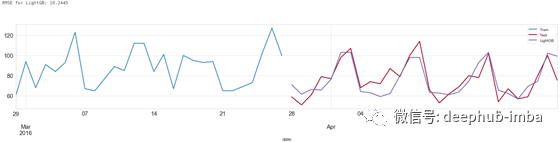
Light Gradient Boosting

model_name='LightGB'
predictions[model_name] = test_final["preds_"+model_name]

#visualize
fig, ax = plt.subplots(figsize=(25,4))
train[-28:].plot(x='date',y='demand',label='Train',ax=ax)
test_final.plot(x='date',y='demand',label='Test',ax=ax);
predictions.plot(x='date',y=model_name,label=model_name,ax=ax);
#evaluate
score = np.sqrt(mean_squared_error(predictions[model_name].values, test_final['demand']))
print('RMSE for {}: {:.4f}'.format(model_name,score))

stats = stats.append({'Model Name':model_name, 'Execution Time':t_lgb, 'RMSE':score},ignore_index=True)

Light Gradient Boosting 预测结果

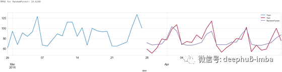
Random Forest

model_name='RandomForest'
predictions[model_name] = test_final["preds_"+model_name]

#visualize
fig, ax = plt.subplots(figsize=(25,4))
train[-28:].plot(x='date',y='demand',label='Train',ax=ax)
test_final.plot(x='date',y='demand',label='Test',ax=ax);
predictions.plot(x='date',y=model_name,label=model_name,ax=ax);
#evaluate
score = np.sqrt(mean_squared_error(predictions[model_name].values, test_final['demand']))
print('RMSE for {}: {:.4f}'.format(model_name,score))

stats = stats.append({'Model Name':model_name, 'Execution Time':t_lgb, 'RMSE':score},ignore_index=True)

Random Forest 预测结果

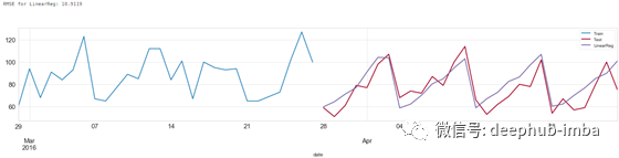
Linear Regression

model_name='LinearReg'
predictions[model_name] = test_final["preds_"+model_name]

#visualize
fig, ax = plt.subplots(figsize=(25,4))
train[-28:].plot(x='date',y='demand',label='Train',ax=ax)
test_final.plot(x='date',y='demand',label='Test',ax=ax);
predictions.plot(x='date',y=model_name,label=model_name,ax=ax);
#evaluate
score = np.sqrt(mean_squared_error(predictions[model_name].values, test_final['demand']))
print('RMSE for {}: {:.4f}'.format(model_name,score))

stats = stats.append({'Model Name':model_name, 'Execution Time':t_linreg, 'RMSE':score},ignore_index=True)

Linear Regression 预测结果

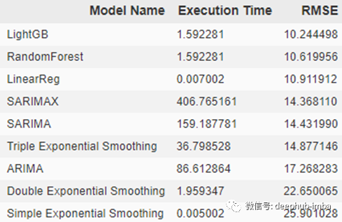
以上就是所有的预测方法及过程。各个方法的运算时间及结果误差如下：

stats.sort_values(by='RMSE')
stats.plot(kind='bar',x='Model Name', y='RMSE', figsize=(12,6), title="Model RMSE Comparison - Lower is better");

各个方法的运算时间及结果误差对比

各个方法的结果误差对比

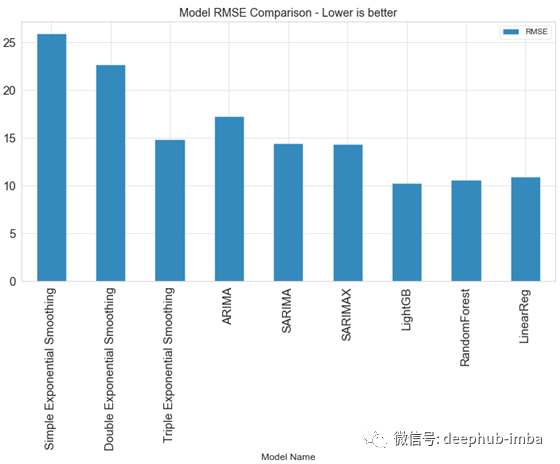
可以看出，传统预测方法的性能相较于机器学习预测方法较差。

但是这个结论并不是绝对的。方法的准确度取决于不同的问题背景。机器学习方法依赖于特征数据。如果我们只有时间序列数据，那么特征数据较为缺乏，我们可以基于原始数据创建特征数据，如滞后数据、移动平均数据等。因此机器学习方法要呈现更好地预测结果，特征工程至关重要。在机器学习领域，某种程度上，数据才是起决定作用，而不是模型或者算法。

本文代码：https://github.com/Deffro/Data-Science-Portfolio/tree/master/Notebooks/Forecasting%20Wars%20-%20Classical%20Forecasting%20Methods%20vs%20Machine%20Learning

作者：Dimitris Effrosynidis

deephub翻译组： Oliver Lee

DeepHub

微信号 : deephub-imba

每日大数据和人工智能的重磅干货

大厂职位内推信息

长按识别二维码关注 ->

好看就点在看！********** **********