车道线检测

前言

目前，车道线检测技术已经相当成熟，主要应用在自动驾驶、智能交通等领域。下面列举一些当下最流行的车道线检测方法：

• 基于图像处理的车道线检测方法。该方法是通过图像处理技术从摄像头传回的图像中提取车道线信息的一种方法，主要是利用图像处理算法进行车道线的检测和识别，并输出车道线的位置信息。
• 基于激光雷达的车道线检测方法。该方法通过激光雷达扫描地面，获取车道线位置信息。这种方法对于在光照较弱、天气恶劣的情况下车道线能更加准确地被检测出来。
• 基于雷达与摄像头的融合车道线检测方法。此方法是将雷达和摄像头两个传感器的数据进行融合，从而得到更加准确的车道线位置信息，检测的鲁棒性也得到了提高。
• 基于GPS和地图的车道线检测方法。该方法主要是利用车辆上的GPS以及地图数据来检测车道线的位置信息。这种方法可以克服图像处理技术在某些特定情况下（比如光照不足或者环境光线无法反射）的不足。

以上这些方法均存在优缺点，不同方法的选择主要取决于具体的技术需求和场景应用。在该章节以基于图像处理的车道线检测方法进行介绍。分别从基础的入门级方法到深度学习的方法进行介绍。

传统图像方法
传统图像方法通过边缘检测滤波等方式分割出车道线区域，然后结合霍夫变换、RANSAC等算法进行车道线检测。这类算法需要人工手动去调滤波算子，根据算法所针对的街道场景特点手动调节参数曲线，工作量大且鲁棒性较差，当行车环境出现明显变化时，车道线的检测效果不佳。基于道路特征检测根据提取特征不同，分为：基于颜色特征、纹理特征、多特征融合；

例如：在车道图像中，路面与车道线交汇处的灰度值变换剧烈，利用边缘增强算子突出图像的局部边缘，定义像素的边缘强度，设置阈值方法提取边缘点；
常用的算子：Sobel算子、Prewitt算子、Log算子、Canny算子；
基于灰度特征检测结构简单，对于路面平整、车道线清晰的结构化道路尤为适用；但当光照强烈、有大量异物遮挡、道路结构复杂、车道线较为模糊时，检测效果受到很大的影响；

使用openCV的传统算法

• Canny边缘检测
• 高斯滤波
• ROI和mask
• 霍夫变换

openCV在图片和视频相关常用的代码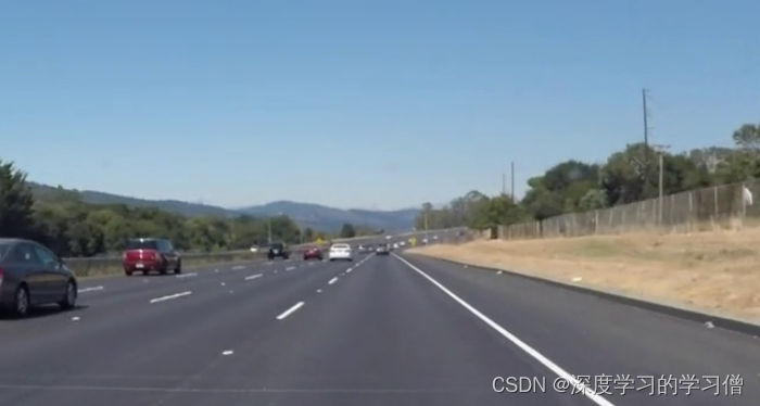

# 读取图片 cv2.imread第一个参数是窗口的名字，第二个参数是读取格式（彩色或灰度）
cv2.imread(const String & filename,int flags = IMREAD_COLOR)#显示图片 cv2.imshow第一个参数是窗口的名字  第二个参数是显示格式，
cv2.imshow(name, img)#保持图片
cv2.imwrite(newfile_name, img)#关闭所有openCV打开的窗口。
cv2.destroyAllWindows()#-----------------------------##打开视频
capture = cv2.VideoCapture('video.mp4')#按帧读取视频 #capture.read()有两个返回值。其中ret是布尔值，如果读取帧是正确的则返回True，如果文件读取到结尾，它的返回值就为False。frame就是每一帧的图像，是个三维矩阵。
ret, frame = capture.read()#视频编码格式设置
fourcc = cv2.VideoWriter_fourcc('X','V','I','D')"""
补充：cv2.VideoWriter_fourcc(‘I’, ‘4’, ‘2’, ‘0’),该参数是YUV编码类型，文件名后缀为.avi
cv2.VideoWriter_fourcc(‘P’, ‘I’, ‘M’, ‘I’),该参数是MPEG-1编码类型，文件名后缀为.avi
cv2.VideoWriter_fourcc(‘X’, ‘V’, ‘I’, ‘D’),该参数是MPEG-4编码类型，文件名后缀为.avi
cv2.VideoWriter_fourcc(‘T’, ‘H’, ‘E’, ‘O’),该参数是Ogg Vorbis,文件名后缀为.ogv
cv2.VideoWriter_fourcc(‘F’, ‘L’, ‘V’, ‘1’),该参数是Flash视频，文件名后缀为.flv
"""

高斯滤波

Canny边缘检测

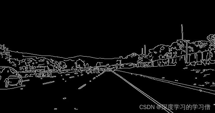
有关边缘检测也是计算机视觉。首先利用梯度变化来检测图像中的边，如何识别图像的梯度变化呢，答案是卷积核。卷积核是就是不连续的像素上找到梯度变化较大位置。我们知道 sobal 核可以很好检测边缘，那么 canny 就是 sobal 核检测上进行优化。
CV2提供了提取图像边缘的函数canny。其算法思想如下：

1. 使用高斯模糊，去除噪音点（cv2.GaussianBlur）
2. 灰度转换（cv2.cvtColor）
3. 使用sobel算子，计算出每个点的梯度大小和梯度方向
4. 使用非极大值抑制(只有最大的保留)，消除边缘检测带来的杂散效应
5. 应用双阈值，来确定真实和潜在的边缘
6. 通过抑制弱边缘来完成最终的边缘检测

#color_img 输入图片#gaussian_ksize 高斯核大小，可以为方形矩阵，也可以为矩形#gaussian_sigmax X方向上的高斯核标准偏差
gaussian = cv2.GaussianBlur(color_img,(gaussian_ksize,gaussian_ksize), gaussian_sigmax)#用于颜色空间转换。input_image为需要转换的图片，flag为转换的类型，返回值为颜色空间转换后的图片矩阵。#flag对应：#cv2.COLOR_BGR2GRAY BGR -> Gray#cv2.COLOR_BGR2RGB BGR -> RGB#cv2.COLOR_BGR2HSV BGR -> HSV
gray_img = cv2.cvtColor(input_image, flag)

输出结果：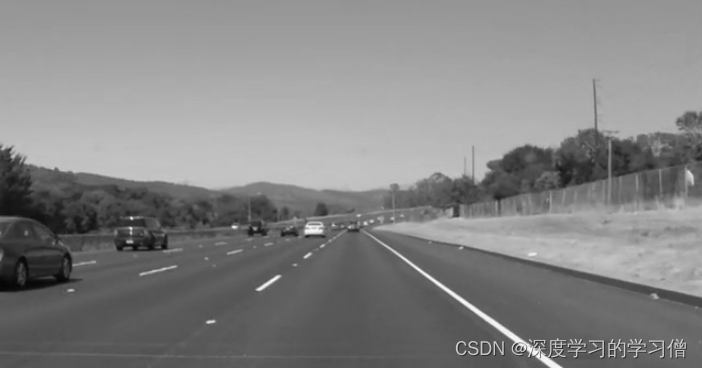

#imag为所操作的图片，threshold1为下阈值，threshold2为上阈值，返回值为边缘图。
edge_img = cv2.Canny(gray_img,canny_threshold1,canny_threshold2)#整成canny_edge_detect的方法defcanny_edge_detect(img):
    gray = cv2.cvtColor(img,cv2.COLOR_RGB2GRAY)
    kernel_size =5
    blur_gray = cv2.GaussianBlur(gray,(kernel_size, kernel_size),0)
    low_threshold =180
    high_threshold =240
    edges = cv2.Canny(blur_gray, low_threshold, high_threshold)return edges

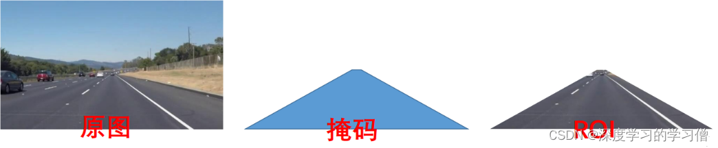
ROI and mask

在机器视觉或图像处理中，通过图像获取到的信息通常是一个二维数组或矩阵，这些信息中可能包含需要进一步处理的区域以及不需要处理的区域。为了提高图像处理的效率和准确性，通常会在需要处理的区域内定义一个感兴趣的区域（ROI），并对该区域进行下一步的处理。ROI可以通过方框、圆、椭圆、不规则多边形等方式勾勒出需要处理的区域。在机器视觉软件中，常常通过图像处理算子和函数来计算ROI。比如，在OpenCV中可以使用cv::Rect、cv::RotatedRect、cv::Point等进行ROI的类型定义和计算；在Matlab中可以使用imrect、imellipse、impoly等函数实现ROI的定义和计算。

处理ROI的目的是为了便于在图像的区域中进行目标检测、物体跟踪、边缘检测、图像分割等操作。通过使用ROI，可以将不需要处理的区域从原始图像中排除掉，从而减少图像处理的复杂度和耗时，提高计算效率和准确性。

#设置ROI和掩码
poly_pts = numpy.array([[[0,368],[300,210],[340,210],[640,368]]])
mask = np.zeros_like(gray_img)
cv2.fillPoly(mask, pts, color)
img_mask = cv2.bitwise_and(gray_img, mask)

霍夫变换

霍夫变换是一种常用的图像处理算法，用于在图像中检测几何形状（如直线、圆、椭圆等）。该算法最初是由保罗·霍夫于 1962 年提出的。简单来说，霍夫变换可以将在直角坐标系中表示的图形转换为极坐标系中的线或曲线，从而方便地进行形状的检测和识别。所以霍夫变换实际上一种由繁到简(类似降维)的操作。在应用中，霍夫变换的过程可以分为以下几个步骤：

1. 针对待检测的形状，选择相应的霍夫曼变换方法。比如，如果要检测直线，可以使用标准霍夫变换；如果要检测圆形，可以使用圆霍夫变换。
2. 将图像转换为灰度图像，并进行边缘检测，以获得待检测的形状目标的轮廓。
3. 以一定的步长和角度范围在霍夫空间中进行投票，将所有可能的直线或曲线与它们可能在的极坐标空间中的位置相对应。
4. 找到霍夫空间中的峰值，这些峰值表示形状的参数空间中存在原始图像中形状的可能性。
5. 通过峰值位置在原始图像中绘制直线、圆等形状。

当使用 canny 进行边缘检测后图像可以交给霍夫变换进行简单图形(线、圆)等的识别。这里用霍夫变换在 canny 边缘检测结果中寻找直线。

# 示例代码，作者丹成学长：Q746876041
mask = np.zeros_like(edges)
    ignore_mask_color =255# 获取图片尺寸
    imshape = img.shape
    # 定义 mask 顶点
    vertices = np.array([[(0,imshape[0]),(450,290),(490,290),(imshape[1],imshape[0])]], dtype=np.int32)# 使用 fillpoly 来绘制 mask
    cv2.fillPoly(mask, vertices, ignore_mask_color)
    masked_edges = cv2.bitwise_and(edges, mask)# 定义Hough 变换的参数
    rho =1 
    theta = np.pi/180
    threshold =2
    min_line_length =4# 组成一条线的最小像素数
    max_line_gap =5# 可连接线段之间的最大像素间距# 创建一个用于绘制车道线的图片
    line_image = np.copy(img)*0# 对于 canny 边缘检测结果应用 Hough 变换# 输出“线”是一个数组，其中包含检测到的线段的端点
    lines = cv2.HoughLinesP(masked_edges, rho, theta, threshold, np.array([]),
                                min_line_length, max_line_gap)# 遍历“线”的数组来在 line_image 上绘制for line in lines:for x1,y1,x2,y2 in line:
            cv2.line(line_image,(x1,y1),(x2,y2),(255,0,0),10)
    color_edges = np.dstack((edges, edges, edges))import math
import cv2
import numpy as np
"""
Gray Scale
Gaussian Smoothing
Canny Edge Detection
Region Masking
Hough Transform
Draw Lines [Mark Lane Lines with different Color]
"""classSimpleLaneLineDetector(object):def__init__(self):passdefdetect(self,img):# 图像灰度处理
        gray_img = self.grayscale(img)print(gray_img)#图像高斯平滑处理
        smoothed_img = self.gaussian_blur(img = gray_img, kernel_size =5)#canny 边缘检测
        canny_img = self.canny(img = smoothed_img, low_threshold =180, high_threshold =240)#区域 Mask
        masked_img = self.region_of_interest(img = canny_img, vertices = self.get_vertices(img))#霍夫变换
        houghed_lines = self.hough_lines(img = masked_img, rho =1, theta = np.pi/180, threshold =20, min_line_len =20, max_line_gap =180)# 绘制车道线
        output = self.weighted_img(img = houghed_lines, initial_img = img, alpha=0.8, beta=1., gamma=0.)return output
    defgrayscale(self,img):return cv2.cvtColor(img, cv2.COLOR_RGB2GRAY)defcanny(self,img, low_threshold, high_threshold):return cv2.Canny(img, low_threshold, high_threshold)defgaussian_blur(self,img, kernel_size):return cv2.GaussianBlur(img,(kernel_size, kernel_size),0)defregion_of_interest(self,img, vertices):
        mask = np.zeros_like(img)iflen(img.shape)>2:
            channel_count = img.shape[2]  
            ignore_mask_color =(255,)* channel_count
        else:
            ignore_mask_color =255
            
        cv2.fillPoly(mask, vertices, ignore_mask_color)
        
        masked_image = cv2.bitwise_and(img, mask)return masked_image
    defdraw_lines(self,img, lines, color=[255,0,0], thickness=10):for line in lines:for x1,y1,x2,y2 in line:
                cv2.line(img,(x1, y1),(x2, y2), color, thickness)defslope_lines(self,image,lines):
        img = image.copy()
        poly_vertices =[]
        order =[0,1,3,2]
        left_lines =[] 
        right_lines =[]for line in lines:for x1,y1,x2,y2 in line:if x1 == x2:passelse:
                    m =(y2 - y1)/(x2 - x1)
                    c = y1 - m * x1
                    if m <0:
                        left_lines.append((m,c))elif m >=0:
                        right_lines.append((m,c))
        left_line = np.mean(left_lines, axis=0)
        right_line = np.mean(right_lines, axis=0)for slope, intercept in[left_line, right_line]:
            rows, cols = image.shape[:2]
            y1=int(rows) 
            y2=int(rows*0.6)
            x1=int((y1-intercept)/slope)
            x2=int((y2-intercept)/slope)
            poly_vertices.append((x1, y1))
            poly_vertices.append((x2, y2))
            self.draw_lines(img, np.array([[[x1,y1,x2,y2]]]))
        
        poly_vertices =[poly_vertices[i]for i in order]
        cv2.fillPoly(img, pts = np.array([poly_vertices],'int32'), color =(0,255,0))return cv2.addWeighted(image,0.7,img,0.4,0.)defhough_lines(self,img, rho, theta, threshold, min_line_len, max_line_gap):"""
        edge_img: 要检测的图片矩阵
        参数2: 距离r的精度,值越大,考虑越多的线
        参数3: 距离theta的精度,值越大,考虑越多的线
        参数4: 累加数阈值,值越小,考虑越多的线
        minLineLength: 最短长度阈值,短于这个长度的线会被排除
        maxLineGap:同一直线两点之间的最大距离
        """
        lines = cv2.HoughLinesP(img, rho, theta, threshold, np.array([]), minLineLength=min_line_len, maxLineGap=max_line_gap)
        line_img = np.zeros((img.shape[0], img.shape[1],3), dtype=np.uint8)
        line_img = self.slope_lines(line_img,lines)return line_img
    defweighted_img(self,img, initial_img, alpha=0.1, beta=1., gamma=0.):
        lines_edges = cv2.addWeighted(initial_img, alpha, img, beta, gamma)return lines_edges
        
    defget_vertices(self,image):
        rows, cols = image.shape[:2]
        bottom_left  =[cols*0.15, rows]
        top_left     =[cols*0.45, rows*0.6]
        bottom_right =[cols*0.95, rows]
        top_right    =[cols*0.55, rows*0.6] 
        
        ver = np.array([[bottom_left, top_left, top_right, bottom_right]], dtype=np.int32)return ver

深度学习方法

• 基于基于分割的方法
• 基于检测的方法
• 基于关键点的方法
• 基于参数曲线的方法

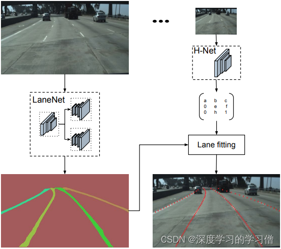
LaneNet+H-Net车道线检测

论文链接：Towards End-to-End Lane Detection: an Instance Segmentation Approach
代码链接

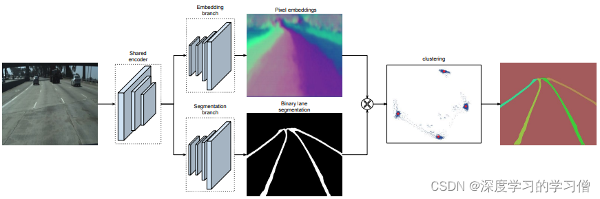
LaneNet+H-Net的车道线检测方法，通过深度学习方法实现端到端的车道线检测，该方法包括两个主要组件，一个是实例分割网络，另一个是车道线检测网络。

该方法的主要贡献在于使用实例分割技术来区分不同车道线之间的重叠和交叉，并且应用多任务学习方法同时实现车道线检测和实例分割。具体来说，该方法将车道线检测问题转化为实例分割问题，使用 Mask R-CNN 实现车道线的分割和检测。通过融合两个任务的 loss 函数，同时对车道线检测和实例分割网络进行训练，实现端到端的车道线检测。

论文中的模型结构主要包括两部分：实例分割网络和车道线检测网络。实例分割网络采用 Mask R-CNN，由主干网络和 Mask R-CNN 网络两部分组成。车道线检测网络采用了 U-Net 结构，用于对掩码图像进行后处理，得到车道线检测结果。

• LaneNet将车道线检测问题转为实例分割问题，即：每个车道线形成独立的实例，但都属于车道线这一类别；H-Net由卷积层和全连接层组成，利用转换矩阵H对同一车道线的像素点进行回归；
• 对于一张输入图片，LaneNet负责输出实例分割结果，每条车道线一个标识ID，H-Net输出一个转换矩阵，对车道线像素点进行修正，并对修正后的结果拟合出一个三阶多项式作为预测的车道线； 测试效果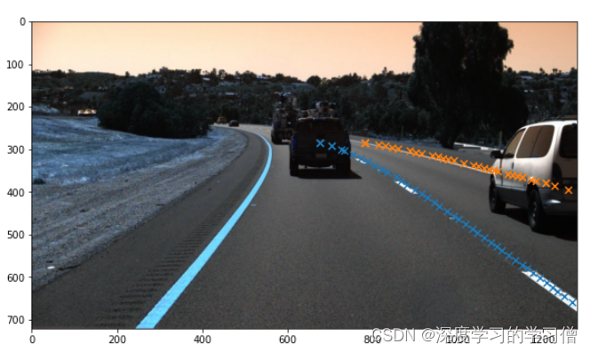

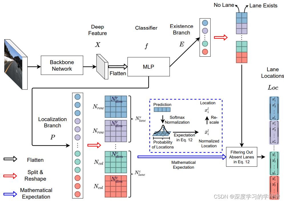
Ultra-Fast-Lane-Detection-V2

论文链接：Ultra Fast Deep Lane Detection with Hybrid Anchor Driven Ordinal Classification
代码：Ultra-Fast-Lane-Detection-V2
![

讲解模型部分的代码

• backbone
• layer
• model_culane
• model_tusimple
• seg_model

backbone

backbone有两类主干方法，VGG和ResNet

• class vgg16bn
• class resnet

import torch,pdb
import torchvision
import torch.nn.modules
class vgg16bn(torch.nn.Module):
    def __init__(self,pretrained = False):
        super(vgg16bn,self).__init__()
        model = list(torchvision.models.vgg16_bn(pretrained=pretrained).features.children())
        model = model[:33]+model[34:43]
        self.model = torch.nn.Sequential(*model)
        
    def forward(self,x):
        return self.model(x)
class resnet(torch.nn.Module):
    def __init__(self,layers,pretrained = False):
        super(resnet,self).__init__()
        #resnet有以下几种选择方式
        if layers == '18':
            model = torchvision.models.resnet18(pretrained=pretrained)
        elif layers == '34':
            model = torchvision.models.resnet34(pretrained=pretrained)
        elif layers == '50':
            model = torchvision.models.resnet50(pretrained=pretrained)
        elif layers == '101':
            model = torchvision.models.resnet101(pretrained=pretrained)
        elif layers == '152':
            model = torchvision.models.resnet152(pretrained=pretrained)
        elif layers == '50next':
            model = torchvision.models.resnext50_32x4d(pretrained=pretrained)
        elif layers == '101next':
            model = torchvision.models.resnext101_32x8d(pretrained=pretrained)
        elif layers == '50wide':
            model = torchvision.models.wide_resnet50_2(pretrained=pretrained)
        elif layers == '101wide':
            model = torchvision.models.wide_resnet101_2(pretrained=pretrained)
        elif layers == '34fca':
            model = torch.hub.load('cfzd/FcaNet', 'fca34' ,pretrained=True)
        else:
            raise NotImplementedError
        
        self.conv1 = model.conv1
        self.bn1 = model.bn1
        self.relu = model.relu
        self.maxpool = model.maxpool
        self.layer1 = model.layer1
        self.layer2 = model.layer2
        self.layer3 = model.layer3
        self.layer4 = model.layer4
    def forward(self,x):
        x = self.conv1(x)
        x = self.bn1(x)
        x = self.relu(x)
        x = self.maxpool(x)
        x = self.layer1(x)
        x2 = self.layer2(x)
        x3 = self.layer3(x2)
        x4 = self.layer4(x3)
        return x2,x3,x4

layer

在这部分代码，是设置网络层的功能模块。其中有两个模块 ： AddCoordinates和CoordConv，它们都是用于卷积操作的。这些模块是用于解决卷积神经网络中的"hole problem"（窟窿问题）的。

• AddCoordinates用于叠加在输入上的坐标信息。具体来说，它将坐标x、y和r(若设置了with_r参数为True)与输入张量相连接。其中，x和y坐标在[-1, 1]范围内进行缩放，坐标原点在中心。r是距离中心的欧几里得距离，并缩放为[0,1]范围内。这样做的目的是为了给卷积层提供额外的位置信息，以便提高其对位置信息的感知。
• CoordConv模块则利用AddCoordinates模块中加入的坐标信息进行卷积操作。在当前张量和坐标信息合并后，将结果输入到卷积层中进行卷积操作。其余参数与torch.nn.Conv2d相同。

需要注意的是，这些模块需要结合使用，AddCoordinates模块在CoordConv模块之前使用，以确保卷积层能够获取到足够的位置信息。

import torch
from torch import nn
classAddCoordinates(object):r"""Coordinate Adder Module as defined in 'An Intriguing Failing of
    Convolutional Neural Networks and the CoordConv Solution'
    (https://arxiv.org/pdf/1807.03247.pdf).
    This module concatenates coordinate information (`x`, `y`, and `r`) with
    given input tensor.
    `x` and `y` coordinates are scaled to `[-1, 1]` range where origin is the
    center. `r` is the Euclidean distance from the center and is scaled to
    `[0, 1]`.
    Args:
        with_r (bool, optional): If `True`, adds radius (`r`) coordinate
            information to input image. Default: `False`
    Shape:
        - Input: `(N, C_{in}, H_{in}, W_{in})`
        - Output: `(N, (C_{in} + 2) or (C_{in} + 3), H_{in}, W_{in})`
    Examples:
        >>> coord_adder = AddCoordinates(True)
        >>> input = torch.randn(8, 3, 64, 64)
        >>> output = coord_adder(input)
        >>> coord_adder = AddCoordinates(True)
        >>> input = torch.randn(8, 3, 64, 64).cuda()
        >>> output = coord_adder(input)
        >>> device = torch.device("cuda:0")
        >>> coord_adder = AddCoordinates(True)
        >>> input = torch.randn(8, 3, 64, 64).to(device)
        >>> output = coord_adder(input)
    """def__init__(self, with_r=False):
        self.with_r = with_r
    def__call__(self, image):
        batch_size, _, image_height, image_width = image.size()
        y_coords =2.0* torch.arange(image_height).unsqueeze(1).expand(image_height, image_width)/(image_height -1.0)-1.0
        x_coords =2.0* torch.arange(image_width).unsqueeze(0).expand(image_height, image_width)/(image_width -1.0)-1.0
        coords = torch.stack((y_coords, x_coords), dim=0)if self.with_r:
            rs =((y_coords **2)+(x_coords **2))**0.5
            rs = rs / torch.max(rs)
            rs = torch.unsqueeze(rs, dim=0)
            coords = torch.cat((coords, rs), dim=0)
        coords = torch.unsqueeze(coords, dim=0).repeat(batch_size,1,1,1)
        image = torch.cat((coords.to(image.device), image), dim=1)return image
classCoordConv(nn.Module):r"""2D Convolution Module Using Extra Coordinate Information as defined
    in 'An Intriguing Failing of Convolutional Neural Networks and the
    CoordConv Solution' (https://arxiv.org/pdf/1807.03247.pdf).
    Args:
        Same as `torch.nn.Conv2d` with two additional arguments
        with_r (bool, optional): If `True`, adds radius (`r`) coordinate
            information to input image. Default: `False`
    Shape:
        - Input: `(N, C_{in}, H_{in}, W_{in})`
        - Output: `(N, C_{out}, H_{out}, W_{out})`
    Examples:
        >>> coord_conv = CoordConv(3, 16, 3, with_r=True)
        >>> input = torch.randn(8, 3, 64, 64)
        >>> output = coord_conv(input)
        >>> coord_conv = CoordConv(3, 16, 3, with_r=True).cuda()
        >>> input = torch.randn(8, 3, 64, 64).cuda()
        >>> output = coord_conv(input)
        >>> device = torch.device("cuda:0")
        >>> coord_conv = CoordConv(3, 16, 3, with_r=True).to(device)
        >>> input = torch.randn(8, 3, 64, 64).to(device)
        >>> output = coord_conv(input)
    """def__init__(self, in_channels, out_channels, kernel_size,
                 stride=1, padding=0, dilation=1, groups=1, bias=True,
                 with_r=False):super(CoordConv, self).__init__()
        in_channels +=2if with_r:
            in_channels +=1
        self.conv_layer = nn.Conv2d(in_channels, out_channels,
                                    kernel_size, stride=stride,
                                    padding=padding, dilation=dilation,
                                    groups=groups, bias=bias)
        self.coord_adder = AddCoordinates(with_r)defforward(self, x):
        x = self.coord_adder(x)
        x = self.conv_layer(x)return x

seg_model

• 主要包含conv_bn_relu和SegHead
• conv_bn_relu模块包含一个卷积层、一个BatchNorm层和ReLU激活函数。这些层的目的是将输入张量x进行卷积、BN和ReLU激活操作，并将结果返回。
• SegHead模块实现了一个带有分支的分割头。它包括三个分支，它们分别对应于主干网络的不同层级。每个分支都由卷积、BN和ReLU激活函数组成，并使用双线性插值对它们的输出进行上采样。然后它们的输出会被拼接在一起，输入到一个包含一系列卷积层的组合中。最后，它输出一个张量，其中包含num_lanes + 1个通道，表示每个车道的掩码以及背景。

import torch
from utils.common import initialize_weights
classconv_bn_relu(torch.nn.Module):def__init__(self,in_channels, out_channels, kernel_size, stride=1, padding=0, dilation=1,bias=False):super(conv_bn_relu,self).__init__()
        self.conv = torch.nn.Conv2d(in_channels,out_channels, kernel_size, 
            stride = stride, padding = padding, dilation = dilation,bias = bias)
        self.bn = torch.nn.BatchNorm2d(out_channels)
        self.relu = torch.nn.ReLU()defforward(self,x):
        x = self.conv(x)
        x = self.bn(x)
        x = self.relu(x)return x
        
classSegHead(torch.nn.Module):def__init__(self,backbone, num_lanes):super(SegHead, self).__init__()
        self.aux_header2 = torch.nn.Sequential(
            conv_bn_relu(128,128, kernel_size=3, stride=1, padding=1)if backbone in['34','18']else conv_bn_relu(512,128, kernel_size=3, stride=1, padding=1),
            conv_bn_relu(128,128,3,padding=1),
            conv_bn_relu(128,128,3,padding=1),
            conv_bn_relu(128,128,3,padding=1),)
        self.aux_header3 = torch.nn.Sequential(
            conv_bn_relu(256,128, kernel_size=3, stride=1, padding=1)if backbone in['34','18']else conv_bn_relu(1024,128, kernel_size=3, stride=1, padding=1),
            conv_bn_relu(128,128,3,padding=1),
            conv_bn_relu(128,128,3,padding=1),)
        self.aux_header4 = torch.nn.Sequential(
            conv_bn_relu(512,128, kernel_size=3, stride=1, padding=1)if backbone in['34','18']else conv_bn_relu(2048,128, kernel_size=3, stride=1, padding=1),
            conv_bn_relu(128,128,3,padding=1),)
        self.aux_combine = torch.nn.Sequential(
            conv_bn_relu(384,256,3,padding=2,dilation=2),
            conv_bn_relu(256,128,3,padding=2,dilation=2),
            conv_bn_relu(128,128,3,padding=2,dilation=2),
            conv_bn_relu(128,128,3,padding=4,dilation=4),
            torch.nn.Conv2d(128, num_lanes+1,1)# output : n, num_of_lanes+1, h, w)
        initialize_weights(self.aux_header2,self.aux_header3,self.aux_header4,self.aux_combine)# self.droput = torch.nn.Dropout(0.1)defforward(self,x2,x3,fea):
        x2 = self.aux_header2(x2)
        x3 = self.aux_header3(x3)
        x3 = torch.nn.functional.interpolate(x3,scale_factor =2,mode='bilinear')
        x4 = self.aux_header4(fea)
        x4 = torch.nn.functional.interpolate(x4,scale_factor =4,mode='bilinear')
        aux_seg = torch.cat([x2,x3,x4],dim=1)
        aux_seg = self.aux_combine(aux_seg)return aux_seg

未完待续！