带图讲解，深度学习YOLO里面的anchors的进阶理解

如果有了解过yolo网络，那肯定也听说过anchors，当然anchors这个概念布置在YOLO里面才有，在其他的目标检测中也存在anchors这个概念。对于anchors计算的一些公式这篇文章就不进行讲解了，这篇文章主要是讲在训练网络模型过程中anchors执行的流程，并将这个抽象的概念具体化，便于更深的理解yolo。

• 1. anchors是什么？

答：anchors其实就是在训练之前人为设定的先验框，网络输出结果的框就是在anchors的基础上进行调整的。所以说先验框设定的好坏对于模型的输出效果影响还是挺大的。在yolo中一般设定一个物体的先验框的个数一般是9个，例如：

anchors = np.array(
    [[27., 183.], [87., 31.], [51., 62.], [139., 95.], [53., 50.], [60., 54.5], [87., 55.], [161., 41.], [49.5, 44.]])

这个先验框anchors一共有9个元素，每一个元素代表一个先验框的宽高。例如【27,183】就表示第一个先验框的宽为27，高为183。

• 2.一张图片有多少个先验框？

答：先验框的个数与图片是哪个的物体的个数有关系，一个物体默认会设定9个先验框。

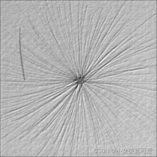
在标注的时候会用一个矩形框来将物体标注出来，这样子我们可以根据标注信息来获取物体的左上角（x1, y1）和右下角(x2,y2)坐标，然后计算出物体的中心坐标[(x2-x1)/2, (y2-y1)/2]。 这样子就可以把ancors表示出来了。下面就是原图与画了先验框的图片的对比：

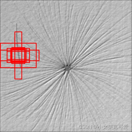
3.先验框在哪一步会进行调整？

答：在YOLO网络里面，一张图片进入模型编码之后会输出三个feature map(特征层），分别用

小特征层(20,20)、中特征层(40,40)和大特征层(80,80)来表示。其中小特征层用于检测大物体，中特征层用于检测中等物体，大特征层用于检测小物体。（因为小特征层的尺寸比较小，也就是压缩的倍数多，小物体经过多次压缩的话在小特征层上面可能就不明显甚至没有，所以小特征用于检测大的物体）。anchors是在特征层上进行调整的，但最开始的anchors是相对于原图的，我们需要将anchors的大小以及物体的中心也对应到feature map上。我们可以从feature map上获取到物体中心以及框的宽高的偏移量offset_x, offset_y, offset_w, offset_h, 然后根据偏移量对先验框进行调整。

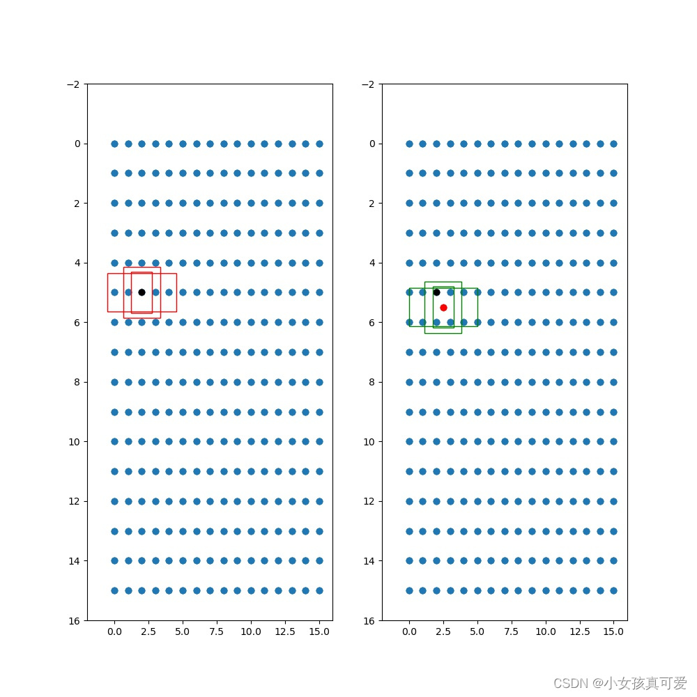
下面是先验框的可视化展示：

原图上：

特征层上：一共9个anchors，有3层特征层， 所以每层3个先验框

左边的红框是先验框没调整之前在特征层上的位置，黑点表示中心位置

右边的绿框是中心点和先验框调整之后在特征层上的位置

opt:懒得打字但又想记录一下的部分。

在训练过程中，对anchors的调整是在求loss前会对anchors进行调整，然后用调整后的anchors和真实框来计算loss_iou。

yolo过了模型之后有三个feature map，所以每个feature map上一个物体有三个anchor，在对anchors进行调整的时候会吧feature map的值调整到0~1之间，这是因为在feature map上每个网格的长度默认为1.

Last:代码实现部分：

代码引用到的YoloDataset, yolo_dataset_collate这两个函数在：

YoloDataset, yolo_dataset_collate：

YoloBody是网络结构，可以用YOLO系列的网络

import os
import random
import cv2
import torch
import numpy as np
from torch.utils.data import DataLoader
import matplotlib.pyplot as plt
from algorithm_code.yolov6.yolo_net import YoloBody
from algorithm_code.yolov6.yolo_dataloader import YoloDataset, yolo_dataset_collate
import os
os.environ["KMP_DUPLICATE_LIB_OK"] = "TRUE"
def sigmoid(x):
    s = 1 / (1 + np.exp(-x))
    return s
def get_anchors_and_decode(feats, anchors, center, num_classes, j):
    feat1 = feats.new(feats.shape)
    feats = feat1.cpu().numpy()
    x, y = center
    plt_w, plt_h = feats.shape[1:3]
    # feats     [batch_size, h, w, 3 * (5 + num_classes)]
    num_anchors = len(anchors)
    grid_shape = np.shape(feats)[1:3]
    #   获得各个特征点的坐标信息。生成的shape为(h, w, num_anchors, 2)
    grid_x = np.tile(np.reshape(np.arange(0, stop=grid_shape[1]), [1, -1, 1, 1]), [grid_shape[0], 1, num_anchors, 1])
    grid_y = np.tile(np.reshape(np.arange(0, stop=grid_shape[0]), [-1, 1, 1, 1]), [1, grid_shape[1], num_anchors, 1])
    grid = np.concatenate([grid_x, grid_y], -1)
    #   将先验框进行拓展，生成的shape为(h, w, num_anchors, 2)
    anchors_tensor = np.reshape(anchors, [1, 1, num_anchors, 2])
    anchors_tensor = np.tile(anchors_tensor, [grid_shape[0], grid_shape[1], 1, 1])
    #   将预测结果调整成(batch_size,h,w,3,nc+5)
    feats = np.reshape(feats, [-1, grid_shape[0], grid_shape[1], num_anchors, num_classes + 5])
    box_xy = sigmoid(feats[..., :2]) + grid
    box_wh = np.exp(feats[..., 2:4]) * anchors_tensor
    fig = plt.figure(figsize=(10., 10.,))
    ax = fig.add_subplot(121)
    plt.ylim(-2, plt_h)
    plt.xlim(-2, plt_w)
    plt.scatter(grid_x, grid_y)
    plt.scatter(x, y, c='black')
    plt.gca().invert_yaxis()
    anchor_left = grid_x - anchors_tensor / 2
    anchor_top = grid_y - anchors_tensor / 2
    print(np.shape(anchor_left))
    rect1 = plt.Rectangle([anchor_left[y, x, 0, 0], anchor_top[y, x, 0, 1]], anchors_tensor[0, 0, 0, 0],
                          anchors_tensor[0, 0, 0, 1], color="r", fill=False)
    rect2 = plt.Rectangle([anchor_left[y, x, 1, 0], anchor_top[y, x, 1, 1]], anchors_tensor[0, 0, 1, 0],
                          anchors_tensor[0, 0, 1, 1], color="r", fill=False)
    rect3 = plt.Rectangle([anchor_left[y, x, 2, 0], anchor_top[y, x, 2, 1]], anchors_tensor[0, 0, 2, 0],
                          anchors_tensor[0, 0, 2, 1], color="r", fill=False)
    ax.add_patch(rect1)
    ax.add_patch(rect2)
    ax.add_patch(rect3)
    ax = fig.add_subplot(122)
    plt.ylim(-2, plt_h)
    plt.xlim(-2, plt_w)
    plt.scatter(grid_x, grid_y)
    plt.scatter(x, y, c='black')
    plt.scatter(box_xy[0, y, x, :, 0], box_xy[0, y, x, :, 1], c='r')
    plt.gca().invert_yaxis()
    pre_left = box_xy[..., 0] - box_wh[..., 0] / 2
    pre_top = box_xy[..., 1] - box_wh[..., 1] / 2
    rect1 = plt.Rectangle([pre_left[0, y, x, 0], pre_top[0, y, x, 0]], box_wh[0, y, x, 0, 0], box_wh[0, y, x, 0, 1],
                          color="g", fill=False)
    rect2 = plt.Rectangle([pre_left[0, y, x, 1], pre_top[0, y, x, 1]], box_wh[0, y, x, 1, 0], box_wh[0, y, x, 1, 1],
                          color="g", fill=False)
    rect3 = plt.Rectangle([pre_left[0, y, x, 2], pre_top[0, y, x, 2]], box_wh[0, y, x, 2, 0], box_wh[0, y, x, 2, 1],
                          color="g", fill=False)
    ax.add_patch(rect1)
    ax.add_patch(rect2)
    ax.add_patch(rect3)
    plt.savefig(r"C:\Users\HJ\Desktop\demo\%s_%s.jpg" % (i, j))
    plt.close()
anchors = np.array(
    [[27., 183.], [87., 31.], [51., 62.], [139., 95.], [53., 50.], [60., 54.5], [87., 55.], [161., 41.], [49.5, 44.]])
anchors_mask = [[6, 7, 8], [3, 4, 5], [0, 1, 2]]
data_line = ['E:/私人文件/V3软件标注/定位/tags/1/1/1_00000001.jpg 42,74,113,289,0 228,236,306,308,1']
train_dataset = YoloDataset(data_line, [512, 512], 10, anchors, False, False)
gen_train = DataLoader(train_dataset, shuffle=True, batch_size=1, num_workers=0, pin_memory=True, drop_last=False,
                       collate_fn=yolo_dataset_collate)
model = YoloBody(num_classes=10).to("cuda")
for iteration, batch in enumerate(gen_train):
    images, targets, y_trues = batch[0], batch[1], batch[2]
    print("image shape:", images.shape)
    boxes = targets[0].cpu().numpy()
    boxes_center = [((box[0] + box[2]) / 2, (box[1] + box[3]) / 2) for box in boxes]
    print("boxes:", boxes_center)
    img_h, img_w = images.shape[2:4]
    print("img_wh:", img_w, img_h)
    with torch.no_grad():
        images = images.to("cuda")
        targets = [ann.to("cuda") for ann in targets]
        y_trues = [ann.to("cuda") for ann in y_trues]
    outputs = model(images)
    for i, feat in enumerate(outputs):
        input_anchor = anchors[anchors_mask[i]]
        # print("input anchor:", input_anchor)
        feat = feat.permute(0, 2, 3, 1)
        print("feat.shape:", feat.shape)
        # 1.获取feat 的高和宽
        feat_h, feat_w = feat.shape[1:3]
        # 2.有了原图大小和feat大小，就可以求出步长
        stride_h, stride_w = img_h / feat_h, img_w / feat_w
        print("stride:", stride_h, stride_w)
        # 3.anchors是相对于原图的，而我们读取数据的到的image是经过resize之后得到的图片,所以我们要先把anchors对应到resize之后的图片，然后再映射到feature map
        # 由于我这里原图是512,512. resize的大小也是512,512所以就不需要将anchor从原图映射到resize之后的图片，也就是少做了一个除法
        feat_anchors = input_anchor / np.array([stride_w, stride_h])  # 把anchors从热size之后的图映射到feature map上
        # 4.根据原图的坐标信息我们可以求出物体的中心位置，有了步长之后局可以求出物体在feature map上面的位置
        for j, center in enumerate(boxes_center):
            feat_x, feat_y = int(center[0] / stride_w), int(center[1] / stride_h)
            print("第%s特征的x, y:" % i, feat_x, feat_y)
            # 5.现在feature map,中心，anchors都有了，就可以画出anchors的图片了
            get_anchors_and_decode(feat, feat_anchors, (feat_x, feat_y), 10, j)
            print("==============================")