【Python气象处理绘图第七弹–泰勒图绘制】

Python气象处理绘图第七弹–泰勒图绘制

泰勒图绘制

前言

在进行模式评估的过程中，常常需要评估模式的模拟性能，这通常由空间相关系数（CC）,相对标准差（SD）及其中心化的均方根误差（RMSE）体现，这三者又常常可以由泰勒图具体体现。RMSE越接近0，CC和SD越接近1，模式模拟能力越好
泰勒图
23.泰勒图

一、数据预处理

对于气象格点数据，其通常为三维数据，但是计算其CC,SD,RMSE时通常需要转成一维数组进行计算。因此需要对气象格点数据进行预处理。

import geopandas as gpd
import salem
# 创造掩膜数据
shp ="E:/shapefile/青藏高原/青藏高原边界数据总集/TPBoundary_HF/TPBoundary_HF_LP.shp"
tp_shp=gpd.read_file(shp)
data0=xr.open_dataset('E:/CORDEX-DOMAIN/conclusion/pr/RX1day.nc')
RX1day=data0.RX1day
data1=xr.open_dataset('E:/CORDEX-DOMAIN/conclusion/pr/RX1day1.nc')
RX1day1=data1.RX1day
data2=xr.open_dataset('E:/CORDEX-DOMAIN/conclusion/pr/RX1day2.nc')
RX1day2=data2.RX1day
data3=xr.open_dataset('E:/CORDEX-DOMAIN/conclusion/pr/RX1day3.nc')
RX1day3=data3.RX1day
RX1day=RX1day.salem.roi(shape=tp_shp)
RX1day1=RX1day1.salem.roi(shape=tp_shp)
RX1day2=RX1day2.salem.roi(shape=tp_shp)
RX1day3=RX1day3.salem.roi(shape=tp_shp)
#将三维数组降为一维
#[数据重组与换形](https://www.jianshu.com/p/3e2eecd6481d)
RX1day=RX1day.stack(z=('time','lat','lon'))
RX1day1=RX1day1.stack(z=('time','lat','lon'))
RX1day2=RX1day2.stack(z=('time','lat','lon'))
RX1day3=RX1day3.stack(z=('time','lat','lon'))
DATA={"RX1day": RX1day,"RX1day1": RX1day1,"RX1day2": RX1day2,"RX1day3": RX1day3,}
df = pd.DataFrame(DATA)
df1=df.dropna(axis=0,subset =["RX1day","RX1day1","RX1day2","RX1day3"])   # 丢弃这四列中有缺失值的行 

二、使用步骤

1.引入库

代码如下（示例）：

from matplotlib.projections import PolarAxes
from mpl_toolkits.axisartist import floating_axes
from mpl_toolkits.axisartist import grid_finder
import numpy as np
import matplotlib.pyplot as plt

2.读入数据

代码如下（示例）：

def set_tayloraxes(fig, location):
    trans = PolarAxes.PolarTransform()
    r1_locs = np.hstack((np.arange(1,10)/10.0,[0.95,0.99]))
    t1_locs = np.arccos(r1_locs)        
    gl1 = grid_finder.FixedLocator(t1_locs)    
    tf1 = grid_finder.DictFormatter(dict(zip(t1_locs,map(str,r1_locs))))
    r2_locs = np.arange(0,2,0.25)
    r2_labels =['0 ','0.25 ','0.50 ','0.75 ','REF ','1.25 ','1.50 ','1.75 ']
    gl2 = grid_finder.FixedLocator(r2_locs)
    tf2 = grid_finder.DictFormatter(dict(zip(r2_locs,map(str,r2_labels))))
    ghelper = floating_axes.GridHelperCurveLinear(trans,extremes=(0,np.pi/2,0,1.75),
                                                  grid_locator1=gl1,tick_formatter1=tf1,
                                                  grid_locator2=gl2,tick_formatter2=tf2)
    ax = floating_axes.FloatingSubplot(fig, location, grid_helper=ghelper)
    fig.add_subplot(ax)
    ax.axis["top"].set_axis_direction("bottom")  
    ax.axis["top"].toggle(ticklabels=True, label=True)
    ax.axis["top"].major_ticklabels.set_axis_direction("top")
    ax.axis["top"].label.set_axis_direction("top")
    ax.axis["top"].label.set_text("Correlation")
    ax.axis["top"].label.set_fontsize(14)
    ax.axis["left"].set_axis_direction("bottom") 
    ax.axis["left"].label.set_text("Standard deviation")
    ax.axis["left"].label.set_fontsize(14)
    ax.axis["right"].set_axis_direction("top")   
    ax.axis["right"].toggle(ticklabels=True)
    ax.axis["right"].major_ticklabels.set_axis_direction("left")
    ax.axis["bottom"].set_visible(False)         
    ax.grid(True)
    polar_ax = ax.get_aux_axes(trans)   
    rs,ts = np.meshgrid(np.linspace(0,1.75,100),
                            np.linspace(0,np.pi/2,100))
    rms = np.sqrt(1+ rs**2-2*rs*np.cos(ts))
    CS = polar_ax.contour(ts, rs,rms,colors='gray',linestyles='--')
    plt.clabel(CS,inline=1, fontsize=10)
    t = np.linspace(0,np.pi/2)
    r = np.zeros_like(t)+1
    polar_ax.plot(t,r,'k--')
    polar_ax.text(np.pi/2+0.032,1.02," 1.00", size=10.3,ha="right", va="top",
                  bbox=dict(boxstyle="square",ec='w',fc='w'))return polar_ax
def plot_taylor(axes, refsample, sample,*args,**kwargs):
    std = np.std(refsample)/np.std(sample)
    corr = np.corrcoef(refsample, sample) 
    theta = np.arccos(corr[0,1])
    t,r = theta,std
    d = axes.plot(t,r,*args,**kwargs)return d

两个函数的使用：

(1) set_tayloraxes(fig, location)

输入：

fig： 需要绘图的figure

location：图的位置，如111为1行1列第一个，122为1行2列第2个

输出：

polar_ax：泰勒坐标系

(2) plot_taylor(axes, refsample, sample, *args, **kwargs)

输入：

axes : setup_axes返回的泰勒坐标系

refsample ：参照样本

sample ：评估样本

args, *kwargs ：plt.plot()函数的相关参数，设置点的颜色，形状等等。

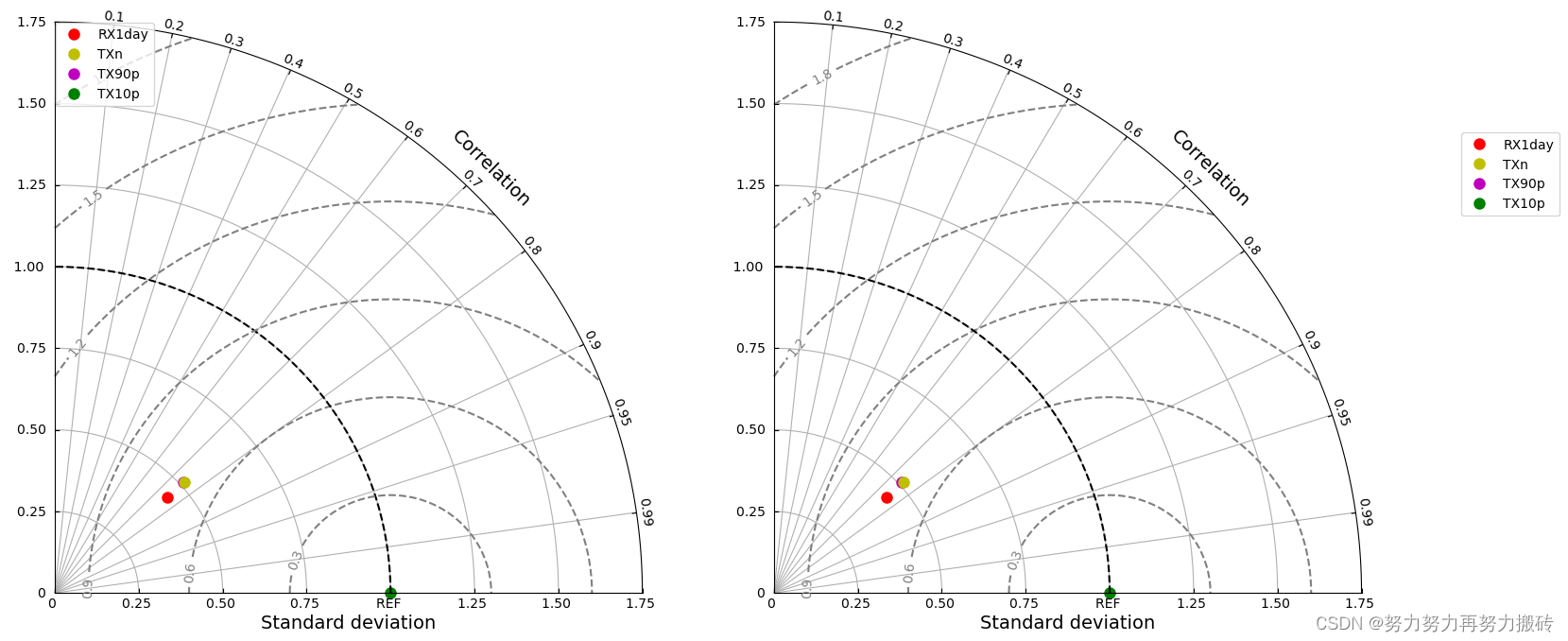
fig = plt.figure(figsize=(12,6))
ax1 =set_tayloraxes(fig,121)
d1 =plot_taylor(ax1,df1.RX1day,df1.RX1day1,'ro',markersize=8,label='RX1day')
d2 =plot_taylor(ax1,df1.RX1day,df1.RX1day2,'yo',markersize=8,label='TXn')
d3 =plot_taylor(ax1,df1.RX1day,df1.RX1day3,'mo',markersize=8,label='TX90p')
d4 =plot_taylor(ax1,df1.RX1day,df1.RX1day,'go',markersize=8,label='TX10p')
ax1.legend(loc=2)
ax2 =set_tayloraxes(fig,122)
d1 =plot_taylor(ax2,df1.RX1day,df1.RX1day1,'ro',markersize=8,label='RX1day')
d2 =plot_taylor(ax2,df1.RX1day,df1.RX1day2,'yo',markersize=8,label='TXn')
d3 =plot_taylor(ax2,df1.RX1day,df1.RX1day3,'mo',markersize=8,label='TX90p')
d4 =plot_taylor(ax2,df1.RX1day,df1.RX1day,'go',markersize=8,label='TX10p')#legend位置
ax2.legend(bbox_to_anchor=(1.32,0.8), borderaxespad=0)

–

总结

以上就是对于泰勒图的绘制。
值得注意的是：

1. 数据预处理成一维数据
2. 剔除缺测值（参考dataframe）df1=df.dropna(axis=0,subset = ["RX1day","RX1day1","RX1day2","RX1day3"])
3. 注意legend的位置Python matplotlib画图时图例说明(legend)放到图像外侧详解