
傅立叶变换是物理学家、数学家、工程师和计算机科学家常用的最有用的工具之一。本篇文章我们将使用Python来实现一个连续函数的傅立叶变换。
我们使用以下定义来表示傅立叶变换及其逆变换。
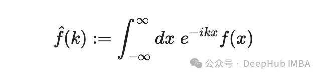
设 f: ℝ → ℂ 是一个既可积又可平方积分的复值函数。那么它的傅立叶变换,记为 f̂,是由以下复值函数给出:
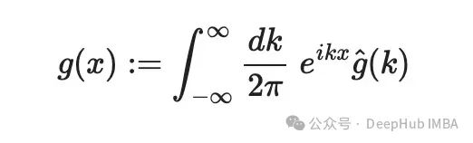
同样地,对于一个复值函数 ĝ,我们定义其逆傅立叶变换(记为 g)为
这些积分进行数值计算是可行的,但通常是棘手的——特别是在更高维度上。所以必须采用某种离散化的方法。
在Numpy文档中关于傅立叶变换如下,实现这一点的关键是离散傅立叶变换(DFT):
当函数及其傅立叶变换都被离散化的对应物所取代时,这被称为离散傅立叶变换(DFT)。离散傅立叶变换由于计算它的一种非常快速的算法而成为数值计算的重要工具,这个算法被称为快速傅立叶变换(FFT),这个算法最早由高斯(1805年)发现,我们现在使用的形式是由Cooley和Tukey公开的
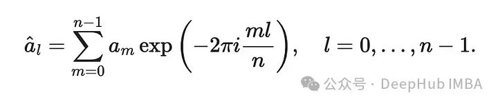
根据Numpy文档,一个具有 n 个元素的序列 a₀, …, aₙ₋₁ 的 DFT 计算如下:
我们将积分分解为黎曼和。在 n 个不同且均匀间隔的点 xₘ = x₀ + m Δx 处对 x 进行采样,其中 m 的范围从 0 到 n-1,x₀ 是任意选择的最左侧点。然后就可以近似表示积分为
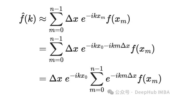
现在对变量 k 进行离散化,在 n 个均匀间隔的点 kₗ = l Δk 处对其进行采样。然后积分变为:
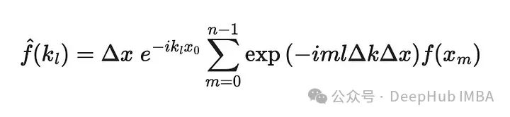
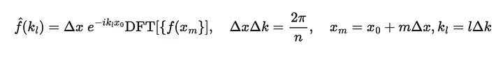
这使得我们可以用类似于 DFT 的形式来计算函数的傅立叶变换。这与DFT的计算形式非常相似,这让我们可以使用FFT算法来高效计算傅立叶变换的近似值。
最后一点是将Δx和Δk联系起来,以便指数项变为-2π I ml/n,这是Numpy的实现方法;
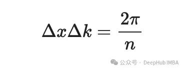
这就是不确定性原理,所以我们得到了最终的方程
我们可以对逆变换做同样的处理。在Numpy中,它被定义为
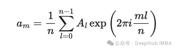
1/n是归一化因子: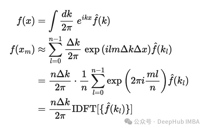
概念和公式我们已经通过Numpy的文档进行了解了,下面开始我们自己的Python实现
 importnumpyasnp
 importmatplotlib.pyplotasplt


 deffourier_transform_1d(func, x, sort_results=False):

     """
     Computes the continuous Fourier transform of function `func`, following the physicist's convention
     Grid x must be evenly spaced.

     Parameters
     ----------

     - func (callable): function of one argument to be Fourier transformed
     - x (numpy array) evenly spaced points to sample the function
     - sort_results (bool): reorders the final results so that the x-axis vector is sorted in a natural order.
         Warning: setting it to True makes the output not transformable back via Inverse Fourier transform

     Returns
     --------
     - k (numpy array): evenly spaced x-axis on Fourier domain. Not sorted from low to high, unless `sort_results` is set to True
     - g (numpy array): Fourier transform values calculated at coordinate k
     """
     x0, dx=x[0], x[1] -x[0]
     f=func(x)

     g=np.fft.fft(f) # DFT calculation

     # frequency normalization factor is 2*np.pi/dt
     w=np.fft.fftfreq(f.size)*2*np.pi/dx

     # Multiply by external factor
     g*=dx*np.exp(-complex(0,1)*w*x0)

     ifsort_results:
         zipped_lists=zip(w, g)
         sorted_pairs=sorted(zipped_lists)
         sorted_list1, sorted_list2=zip(*sorted_pairs)
         w=np.array(list(sorted_list1))
         g=np.array(list(sorted_list2))

     returnw, g


 definverse_fourier_transform_1d(func, k, sort_results=False):
     """
     Computes the inverse Fourier transform of function `func`, following the physicist's convention
     Grid x must be evenly spaced.

     Parameters
     ----------

     - func (callable): function of one argument to be inverse Fourier transformed
     - k (numpy array) evenly spaced points in Fourier space to sample the function
     - sort_results (bool): reorders the final results so that the x-axis vector is sorted in a natural order.
         Warning: setting it to True makes the output not transformable back via Fourier transform

     Returns
     --------
     - y (numpy array): evenly spaced x-axis. Not sorted from low to high, unless `sort_results` is set to True
     - h (numpy array): inverse Fourier transform values calculated at coordinate x
     """
     dk=k[1] -k[0]

     f=np.fft.ifft(func) *len(k) *dk/(2*np.pi)
     x=np.fft.fftfreq(f.size)*2*np.pi/dk

     ifsort_results:
         zipped_lists=zip(x, f)
         sorted_pairs=sorted(zipped_lists)
         sorted_list1, sorted_list2=zip(*sorted_pairs)
         x=np.array(list(sorted_list1))
         f=np.array(list(sorted_list2))
     returnx, f
我们来通过一些例子看看我们自己实现是否正确。
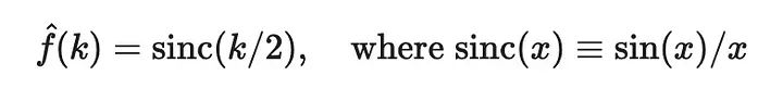
第一个例子:阶跃函数
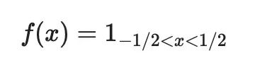
函数在-1/2和1/2之间是1,在其他地方是0。它的傅里叶变换是
N = 2048
# Define the function f(x)
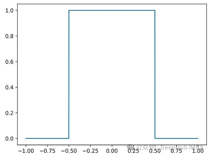
f = lambda x: np.where((x >= -0.5) & (x <= 0.5), 1, 0)
x = np.linspace(-1, 1, N)
plt.plot(x, f(x));
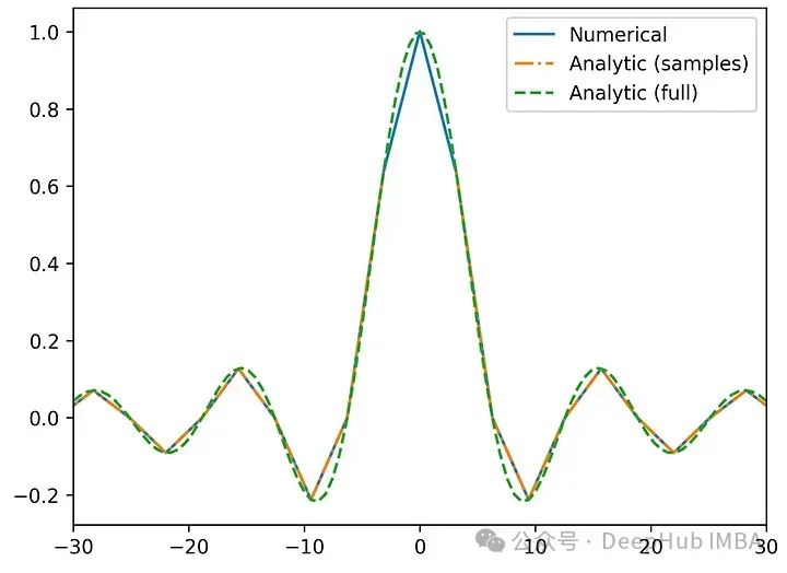
画出傅里叶变换,以及在k的采样值和整个连续体上计算的解析解:
 k, g = fourier_transform_1d(f, x, sort_results=True) # make it easier to plot
 kk = np.linspace(-30,30, 100)

 plt.plot(k, np.real(g), label='Numerical');
 plt.plot(k, np.sin(k/2)/(k/2), linestyle='-.', label='Analytic (samples)')
 plt.plot(kk, np.sin(kk/2)/(kk/2), linestyle='--', label='Analytic (full)')
 plt.xlim(-30, 30)
 plt.legend();
看起来是没问题的,然后我们把它转换回来:
 k, g = fourier_transform_1d(f, x)
 y, h = inverse_fourier_transform_1d(g, k, sort_results=True)

 plt.plot(y, np.real(h), label='Numerical transform')
 plt.plot(x, f(x), linestyle='--', label='Analytical')
 plt.legend();
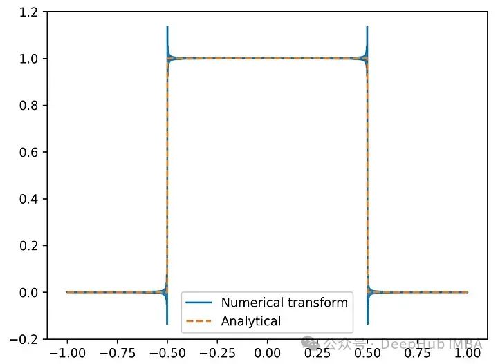
我们可以清楚地看到不连续边缘处的 Gibbs 现象——这是傅里叶变换的一个预期特征。
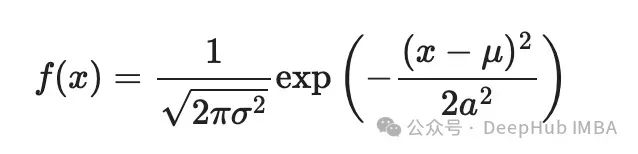
第二个例子:高斯PDF
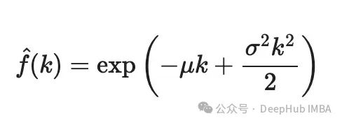
傅里叶变换
下面,我们绘制数值傅里叶变换和解析值: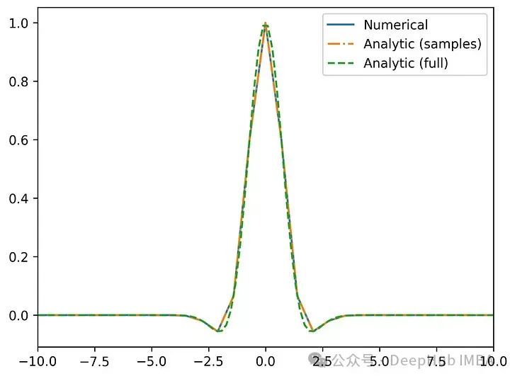
以及傅里叶逆变换与原函数的对比
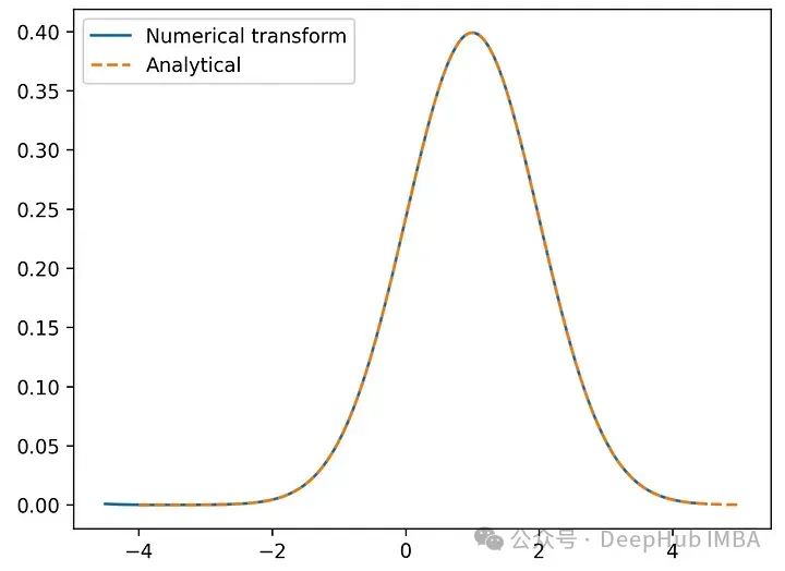
可以看到,我们的实现没有任何问题
最后,如果你对机器学习的基础计算和算法比较感兴趣,可以多多关注Numpy和SK-learn的文档(还有scipy但是这个更复杂),这两个库不仅有很多方法的实现,还有这些方法的详细解释,这对于我们学习是非常有帮助的。
例如本文的一些数学的公式和概念就是来自于Numpy的文档,有兴趣的可以直接看看
https://numpy.org/doc/stable/reference/routines.fft.html
作者:Alessandro Morita Gagliardi