
👦👦一个帅气的boy,你可以叫我Love And Program
🖱 ⌨个人主页:Love And Program的个人主页
💖💖如果对你有帮助的话希望三连💨💨支持一下博主
降维实操
前言
最近看书看到降维一部分,说实话这一部分一直想写,但是苦于网上讲解的初级理论部分过于全面,自己也是无从可写,但看完周志华的机器学习一书中写的降维部分,感觉还是有新的理解的,权当记录一下,文中有什么不对的地方还望大佬们多担待,评论我我会及时更改。
线性降维
降维是将数据通过某种数学变换将原始高维属性空间转变为一个低维“子空间”,在此子空间中样本密度大幅提高,距离计算也变得更为容易,通俗点讲就是关系更加密切,训练模型鲁棒性更好。
低维嵌入
这样就引出了我们为什么要将数据降维的原因,实际任务中人们收集或观测的数据样本是高维的,但是与学习任务密切相关的也许仅仅是某个低维分布,即**高维空间中的一个低维“嵌入”**,在这个低维嵌入子空间中更容易让模型学习。
多维缩放(MDS)
简介
在原始空间中样本之间的距离在低维空间中得以保持即得到“多维缩放”(MDS),其采用欧氏距离计算原始空间中的距离,尽可能保留高维空间中的“相似度”信息。
算法描述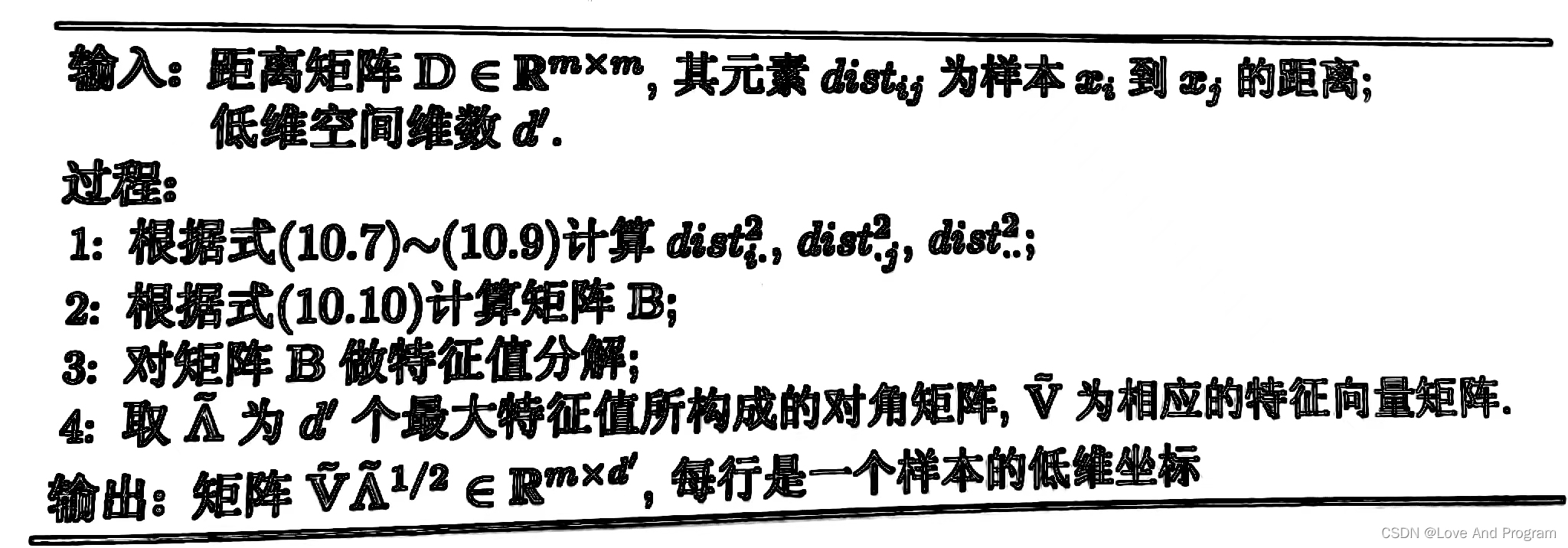
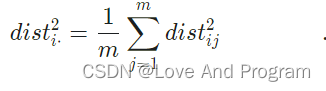
式(10.7)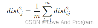
式(10.8)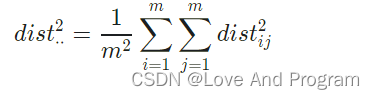
式(10.9)
式(10.10)
推导可见
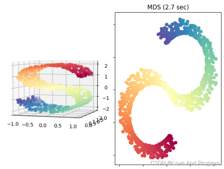
MDS示例代码
from collections import OrderedDict
from functools import partial
from time import time

import matplotlib.pyplot as plt
from mpl_toolkits.mplot3d import Axes3D
from matplotlib.ticker import NullFormatter
from sklearn import manifold, datasets
Axes3D

n_points =1000
X, color = datasets.make_s_curve(n_points, random_state=0)
fig = plt.figure()

ax = fig.add_subplot(121, projection='3d')
ax.scatter(X[:,0], X[:,1], X[:,2], c=color, cmap=plt.cm.Spectral)
ax.view_init(4,-72)
methods = OrderedDict()
methods['MDS']= manifold.MDS(n_components, max_iter=100, n_init=1)for i,(label, method)inenumerate(methods.items()):
    t0 = time()
    Y = method.fit_transform(X)
    t1 = time()print("%s: %.2g sec"%(label, t1 - t0))
    ax = fig.add_subplot(1,2,2)
    ax.scatter(Y[:,0], Y[:,1], c=color, cmap=plt.cm.Spectral)
    ax.set_title("%s (%.2g sec)"%(label, t1 - t0))
    ax.xaxis.set_major_formatter(NullFormatter())
    ax.yaxis.set_major_formatter(NullFormatter())
    ax.axis('tight')
plt.show()
主成分分析法
简介
   主成分分析(Principal Component Analysis,PCA), 是一种统计方法,通过正交变换将一组可能存在相关性的变量转换为一组线性不相关的变量,转换后的这组变量叫主成分(来源于百度百科)。
    主成分分析法适用于变量间有较强相关性的数据,毕竟数据间关系弱的,经过PCA降维后会舍弃部分信息,关系可能会更弱,那用降维的意义也就不存在了,其具体作用有两方面:
- 舍弃此部分信息后能使样本的采样密度增大,正如上面所说:高维数据到低维数据转换后数据间的密度会大大提高;
- 当数据受到噪声影响时,最小的特征值所对应的特征向量往往与噪声有关,将它们舍弃可以在一定程度上起到去噪的效果;
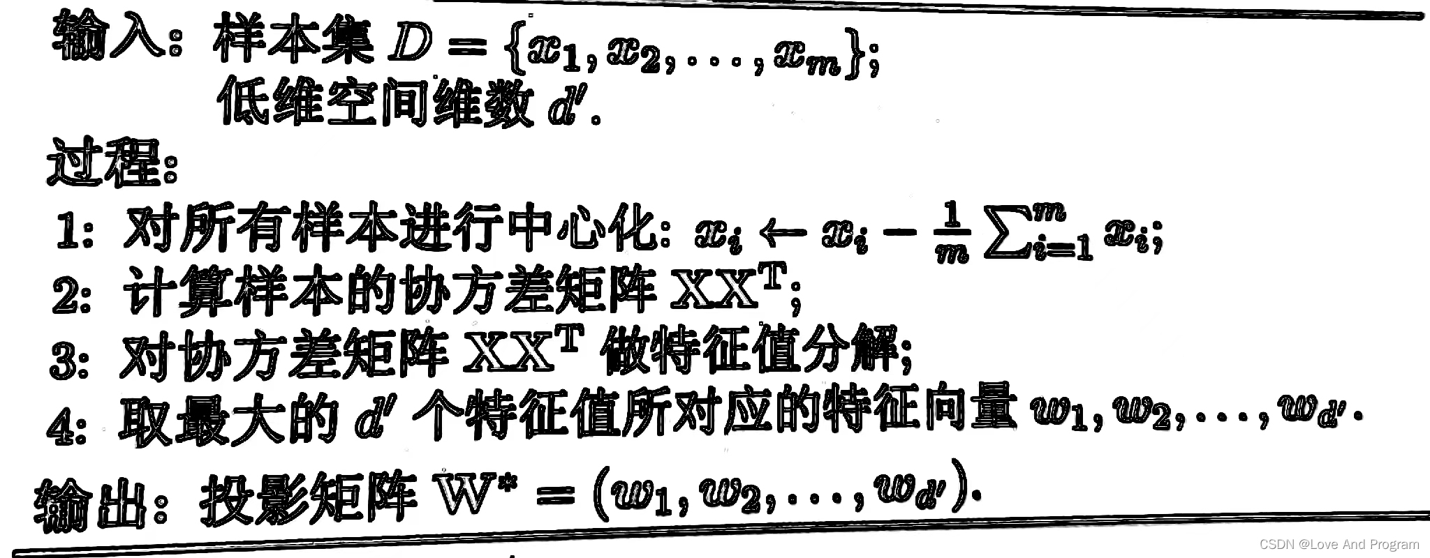
算法描述
核化线性降维
简介
核化线性降维是非线性降维,是基于核技巧对线性降维方法进行“核化”,例如核主成分分析(KPCA),优点就是,保留了最主要的特征,计算方法简单,但缺点也很明显,使用非线性核可以实现非线性降维计算开销极大,直接给我报Memory Error,以下代码请酌情更改输入数据集比例。
PCA和KPCA手写数字体识别实例代码
from sklearn.model_selection import train_test_split
import pandas as pd
from sklearn.decomposition import KernelPCA
from sklearn.datasets import fetch_openml
mnist = fetch_openml('mnist_784', cache=True)print(mnist.data.shape)import matplotlib.pyplot as plt
defdisplay_sample(num):

    image = mnist.data.iloc[num,:].to_numpy().reshape([28,28])
    plt.imshow(image, cmap=plt.get_cmap('gray_r'))
    plt.show()
display_sample(10)

train_img, test_img, train_lbl, test_lbl = train_test_split(
    mnist.data, mnist.target, test_size=0.8, random_state=0)print(train_img.shape)print(test_img.shape)from sklearn.preprocessing import StandardScaler
scaler = StandardScaler()
scaler.fit(train_img)
train_img = scaler.transform(train_img)
test_img = scaler.transform(test_img)from sklearn.linear_model import LogisticRegression
logisticRegr = LogisticRegression(solver ='lbfgs',max_iter=1000)
logisticRegr.fit(train_img, train_lbl)
score = logisticRegr.score(test_img, test_lbl)print(score)# KPCA# scikit_kpca = KernelPCA(n_components=2, kernel='rbf', gamma=15)# X_skernpca = scikit_kpca.fit_transform(train_img)# plt.scatter(X_skernpca[test_img, 0], X_skernpca[test_img, 1], color='red', marker='^', alpha=0.5)# plt.scatter(X_skernpca[test_lbl, 0], X_skernpca[test_lbl==1, 1], color='blue', marker='o', alpha=0.5)# plt.xlabel('PC1')# plt.ylabel('PC2')# plt.tight_layout()# plt.show()# PCAfrom sklearn.decomposition import PCA
pca = PCA(0.95)
pca.fit(train_img)print(pca.n_components_)
train2_img = pca.transform(train_img)
test2_img = pca.transform(test_img)print(train2_img.shape)print(train_img.shape)

logisticRegr = LogisticRegression(solver ='lbfgs',max_iter=1000)
logisticRegr.fit(train2_img, train_lbl)
score = logisticRegr.score(test2_img, test_lbl)print(score)#minist数据集及划分比例#(70000, 784)#(14000, 784)#(56000, 784)#降维前预测准确率#0.8843214285714286#保留特征数量#293#降维后数据量对比#(14000, 293)#(14000, 784)#降维后预测准确率#0.9033214285714286
流形学习
简介
流形学习是一类借鉴拓扑流形概念的降维方法,“流形”是在局部与欧氏空间同胚的空间,也就是说他在局部具有欧氏空间的性质,能用欧氏距离来进行距离计算,用到降维中,即低维流形嵌入到高维空间中,局部仍然具有欧氏空间的性质,因此很容易在局部建立降维映射关系,然后在设法将局部映射关系推广到全局,以两种著名的流形学习方法为例,即非线性降维。
等度量映射(Isomap)
Isomap算法是最早的流形学习方法之一,它是等距映射的缩写。Isomap可以看作是多维尺度分析(MDS)或核主成分分析的扩展。
简介
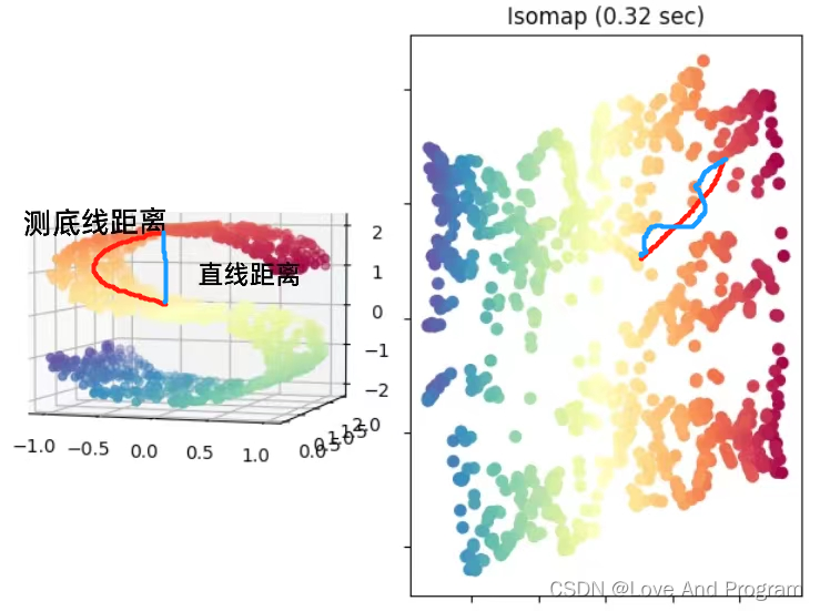
Isomap寻求一种更低维度的嵌入,以保持所有点之间的测地线距离,毕竟如下左图最上面一层到中间一层在三维坐标中不能直接计算直线距离,这样是不恰当的,需要沿着两层之间的边边连线形成距离最短的路径,也就是测地线距离,虽然低维嵌入流形上的测地线距离不能用高维空间的直线距离计算,但是可以通过近邻距离来求近似(图画的不是很好,右图线都是直的嗷,蓝线:近邻距离,也就是左图三维直线距离被二维可视化;红线:测地线距离)
算法描述
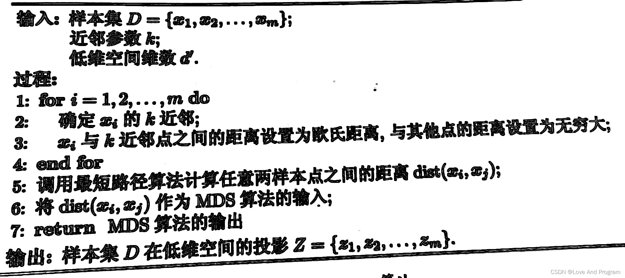
Isomap示例代码
from collections import OrderedDict
from functools import partial
from time import time
import matplotlib.pyplot as plt
from mpl_toolkits.mplot3d import Axes3D
from matplotlib.ticker import NullFormatter
from sklearn import manifold, datasets
# Next line to silence pyflakes. This import is needed.
Axes3D
n_points =1000
X, color = datasets.make_s_curve(n_points, random_state=0)
fig = plt.figure()
ax = fig.add_subplot(121, projection='3d')
ax.scatter(X[:,0], X[:,1], X[:,2], c=color, cmap=plt.cm.Spectral)
ax.view_init(4,-72)
methods = OrderedDict()
methods['Isomap']= manifold.Isomap(n_components=2)for i,(label, method)inenumerate(methods.items()):
    t0 = time()
    Y = method.fit_transform(X)
    t1 = time()print("%s: %.2g sec"%(label, t1 - t0))
    ax = fig.add_subplot(1,2,2)
    ax.scatter(Y[:,0], Y[:,1], c=color, cmap=plt.cm.Spectral)
    ax.set_title("%s (%.2g sec)"%(label, t1 - t0))
    ax.xaxis.set_major_formatter(NullFormatter())
    ax.yaxis.set_major_formatter(NullFormatter())
    ax.axis('tight')

plt.show()
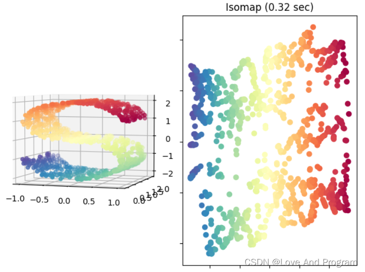
以S型曲线数据集为例,将三维数据映射到二维平面上,如下图所示:
局部线性嵌入(LLE)
简介
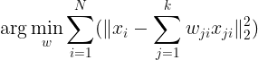
局部线性嵌入试图保持邻域内样本线性关系,意思就是经历过降维后仍然在原空间具有该特征。并且LLE可以在sklearn机器学习库中直接调用。
算法描述: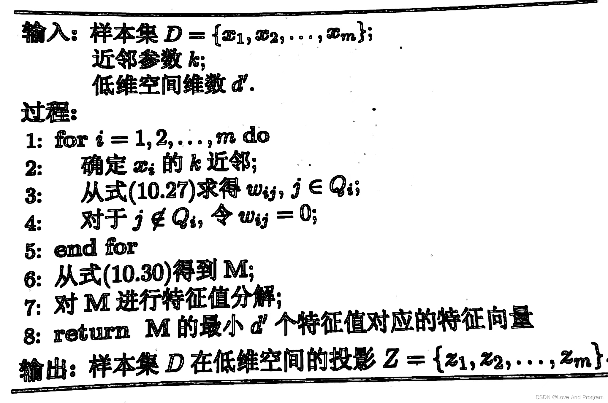
式(10.27)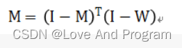 式(10.30)
推导过程(感兴趣可以去看看)
LLE示例代码
import matplotlib.pyplot as plt
from mpl_toolkits.mplot3d import Axes3D
Axes3D
from sklearn import manifold, datasets
X, color = datasets.make_swiss_roll(n_samples=1500)print("Computing LLE embedding")
X_r, err = manifold.locally_linear_embedding(X, n_neighbors=12,
                                             n_components=2)print("Done. Reconstruction error: %g"% err)
fig = plt.figure()

ax = fig.add_subplot(211, projection='3d')
ax.scatter(X[:,0], X[:,1], X[:,2], c=color, cmap=plt.cm.Spectral)

ax.set_title("Original data")
ax = fig.add_subplot(212)
ax.scatter(X_r[:,0], X_r[:,1], c=color, cmap=plt.cm.Spectral)
plt.axis('tight')
plt.xticks([]), plt.yticks([])
plt.title('Projected data')
plt.show()
以swiss(称他为瑞士卷)为例,将三维数据进行二维化: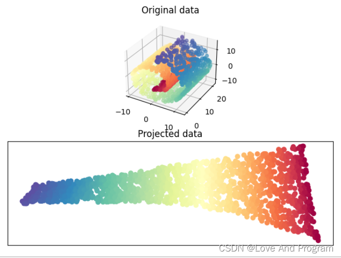
本文转载自: https://blog.csdn.net/qq_43604989/article/details/127958420
版权归原作者 Love And Program 所有, 如有侵权,请联系我们删除。
版权归原作者 Love And Program 所有, 如有侵权,请联系我们删除。