
1.特性
- 即插即用
- 在特征提取效果显著
- 微调模型的小技巧
2.核心思想
- 本质上与人类视觉选择性注意力机制类似,从众多信息中选出对当前任务目标更为关键的信息。
- 通过手段获取每张特征图重要性的差异
- 抑制无用信息,凸显有用信息(将注意力集中在图中重要区域)
3.广泛应用
- 自然语言处理
- 图像识别
- 语音识别
4.卷积神经网络中注意力机制研究现状
4.1单路注意力:
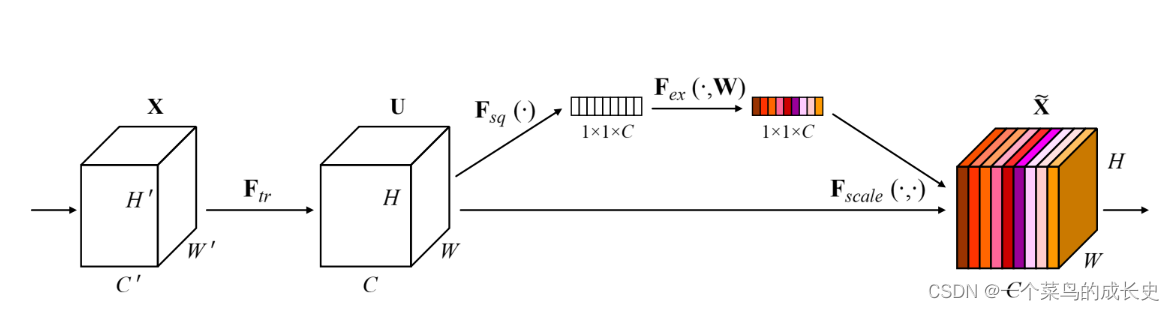
1.SE-Net(Squeeze and Excitation)(2018年CVPR提出):利用注意力机制思想,显式地建模特征图之间的相互依赖关系,并通过学习的方式来自适应地获取到每张特征图的重要性,然后依照这个重要程度去对原数据进行更新。提升有用的特征重要程度同时降低无用特征的重要性,并以不同通道的重要性为指导,将计算资源合理地投入不同通道当中。
- ** 步骤解析如下:**
- 基础的卷积操作:提取特征图
,得到 C个大小为 H*W的feature map。公式如下:
ps:Vc表示第c个卷积核,Xs表示第s个输入
- Squeeze操作:全局平均池化将HWC的输入——变成11C的输出
ps:此步骤表明该层C个Feature map的数值分布情况(全局信息),是分别在某个channel的 feature map中操作。
- Excitation操作:W1z全连接层操作,CC/r (r:缩放参数,目的是减少channel个数降低计算量),W1z维度:11C/r,再经过一个ReLU层,维度不变。再与W2相乘,同样也是一个全连接层操作:W2维度 C/rC,输出维度为11C,经过sigmoid函数,得到s。
ps:s维度 1*1*C,s是用于刻画U中feature map的权重,σ为relu激活函数,δ代表sigmoid激活 函数。
- Uc是一个二维矩阵,Sc是一个数即权重,因此相当于把Uc矩阵中的每个值都乘以Sc。
** 缺点:降维对通道注意预测带来了副作用,捕获所有通道之间的依赖是低效的,也是不必要的。**
** 只注重通道内部信息的综合,没有考虑到相邻信道信息的重要性。**
2.ECA-Net(Efficient Channel Attention)(2020CVPR提出,对SE-Net的改进):不降低通道维数来进行跨通道信息交互的ECA模块。具体如下图所示:
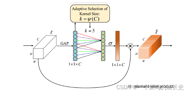
创新点:
- 将SEBlock中MLP模块(FC->ReLU>FC->Sigmoid),转变为一维卷积的形式,有效减少了参数计算量。
- 一维卷积自带的功效就是非全连接,每一次卷积过程只和部分通道的作用,即实现了适当的跨通道交互而不是像全连接层一样全通道交互。
代码实现:
class eca_layer(nn.Module):
    def __init__(self, channel, k_size=3):
        super(eca_layer, self).__init__()
        self.avg_pool = nn.AdaptiveAvgPool2d(1)
        self.conv = nn.Conv1d(1, 1, kernel_size=k_size, padding=(k_size - 1) // 2, bias=False)
        self.sigmoid = nn.Sigmoid()

    def forward(self, x):
        # x: input features with shape [b, c, h, w]
        b, c, h, w = x.size()

        # feature descriptor on the global spatial information
        y = self.avg_pool(x)

        # Two different branches of ECA module
        y = self.conv(y.squeeze(-1).transpose(-1, -2)).transpose(-1, -2).unsqueeze(-1)

        # Multi-scale information fusion
        y = self.sigmoid(y)

        return x * y.expand_as(x)
SE-Net对比ECA-Net:
# SEBlock 采用全连接层方式
def forward(self, x):
    b, c, _, _ = x.shape
    v = self.global_pooling(x).view(b, c)
    v = self.fc_layers(v).view(b, c, 1, 1)
    v = self.sigmoid(v)
    return x * v

# ECABlock 采用一维卷积方式
def forward(self, x):
    v = self.avg_pool(x)
    v = self.conv(v.squeeze(-1).transpose(-1, -2)).transpose(-1, -2).unsqueeze(-1)
    v = self.sigmoid(v)
    return x * v
4.2多路注意力
1.SK-Net
2.Res-Net
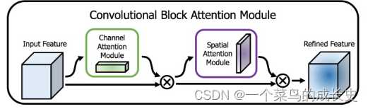
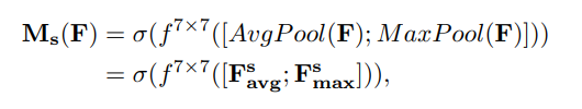
**3.CBAM(Convolutional Block Attention Module)(2018ECCV):**对于卷积网络中的特征图而言,不仅通道蕴含着丰富的注意力信息,通道内部:即特征图像素点间也具有大量的注意力信息,以往注意力只关注通道,不关注空间。因而构建2个子模块,空间注意力SAM(Spatial Attention Module),通道注意力模块CAM(Channel Attention Module)汇总空间和通道两方面的注意力信息,并进行综合,获得更全面可靠的注意力信息。
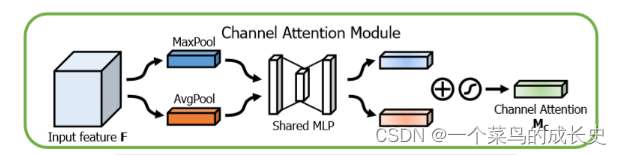
- CAM:1.特征图HWC 经过 MaxPool+AvgPool 得到11C特征图;2.输入两层MLP神经网络:第一层神经元个数C/r(r为缩放率),激活函数ReLU,第二层神经元个数C,激活函数sigmoid。3.element-wise的加和操作,再经过sigmoid激活操作,生成最终的通道注意力特征。
- SAM:1.空间注意力模块将通道注意力模块输出的特征图F作为本模块的输入特征图,特征图HWC 经过基于通道的 MaxPool+AvgPool 得到2个HW1的特征图,基于通道进行拼接;2.经过一个77卷积操作,降维为HW*1,再经过sigmoid生成空间注意力特征。3.最后将该向量和该模块的输入特征图做乘操作,得到最终生成的特征。

代码实现:先通道后空间效果好
class ChannelAttention(nn.Module):
    def __init__(self, in_planes, ratio=16):
        super(ChannelAttention, self).__init__()
        self.avg_pool = nn.AdaptiveAvgPool2d(1)
        self.max_pool = nn.AdaptiveMaxPool2d(1)

        self.fc1 = nn.Conv2d(in_planes, in_planes // ratio, 1, bias=False)
        self.relu1 = nn.ReLU()
        self.fc2 = nn.Conv2d(in_planes // ratio, in_planes, 1, bias=False)
        self.sigmoid = nn.Sigmoid()

    def forward(self, x):
        avg_out = self.fc2(self.relu1(self.fc1(self.avg_pool(x))))
        max_out = self.fc2(self.relu1(self.fc1(self.max_pool(x))))
        out = avg_out + max_out
        return self.sigmoid(out)

class SpatialAttention(nn.Module):
    def __init__(self, kernel_size=7):
        super(SpatialAttention, self).__init__()

        assert kernel_size in (3, 7), 'kernel size must be 3 or 7'
        padding = 3 if kernel_size == 7 else 1

        self.conv1 = nn.Conv2d(2, 1, kernel_size, padding=padding, bias=False)  # 7,3     3,1
        self.sigmoid = nn.Sigmoid()

    def forward(self, x):
        avg_out = torch.mean(x, dim=1, keepdim=True)
        max_out, _ = torch.max(x, dim=1, keepdim=True)
        x = torch.cat([avg_out, max_out], dim=1)
        x = self.conv1(x)
        return self.sigmoid(x)

class CBAM(nn.Module):
    def __init__(self, in_planes, ratio=16, kernel_size=7):
        super(CBAM, self).__init__()
        self.ca = ChannelAttention(in_planes, ratio)
        self.sa = SpatialAttention(kernel_size)

    def forward(self, x):
        out = x * self.ca(x)
        result = out * self.sa(out)
        return result
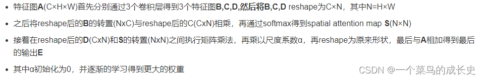
4.双注意力网络DA-Net(CVPR2019):类似于CBAM,综合考虑通道和空间两路的注意力信息。但是获取注意力信息的方式不同,CBAM串行获取两路注意力信息的,而DA-Net是采用并行两路获取注意力信息的。
- PAM 位置注意力
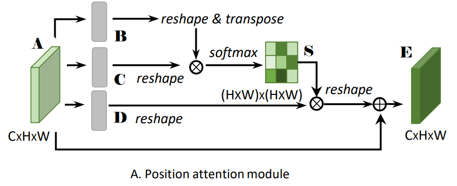
- 具体步骤
- CAM通道注意力
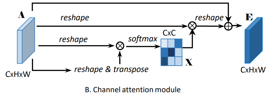
- 具体步骤
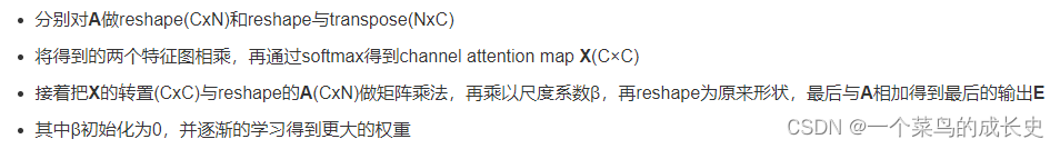
- 代码实现
class PAM_Module(Module):
    def __init__(self, in_dim):
        super(PAM_Module, self).__init__()
        self.chanel_in = in_dim
        # 先经过3个卷积层生成3个新特征图B C D (尺寸不变)
        self.query_conv = Conv2d(in_channels=in_dim, out_channels=in_dim//8, kernel_size=1)
        self.key_conv = Conv2d(in_channels=in_dim, out_channels=in_dim//8, kernel_size=1)
        self.value_conv = Conv2d(in_channels=in_dim, out_channels=in_dim, kernel_size=1)
        self.gamma = Parameter(torch.zeros(1))  # α尺度系数初始化为0,并逐渐地学习分配到更大的权重
        self.softmax = Softmax(dim=-1)  # 对每一行进行softmax
    def forward(self, x):
        m_batchsize, C, height, width = x.size()
        proj_query = self.query_conv(x).view(m_batchsize, -1, width*height).permute(0, 2, 1)
        # C -> (N,C,HW)
        proj_key = self.key_conv(x).view(m_batchsize, -1, width*height)
        # BC,空间注意图 -> (N,HW,HW)
        energy = torch.bmm(proj_query, proj_key)
        # S = softmax(BC) -> (N,HW,HW)
        attention = self.softmax(energy)
        # D -> (N,C,HW)
        proj_value = self.value_conv(x).view(m_batchsize, -1, width*height)
        # DS -> (N,C,HW)
        out = torch.bmm(proj_value, attention.permute(0, 2, 1))  # torch.bmm表示批次矩阵乘法
        # output -> (N,C,H,W)
        out = out.view(m_batchsize, C, height, width)

        out = self.gamma*out + x
        return out


class CAM_Module(Module):
    """ Channel attention module"""
    def __init__(self, in_dim):
        super(CAM_Module, self).__init__()
        self.chanel_in = in_dim
        self.gamma = Parameter(torch.zeros(1))  # β尺度系数初始化为0,并逐渐地学习分配到更大的权重
        self.softmax  = Softmax(dim=-1)  # 对每一行进行softmax
    def forward(self,x):
        m_batchsize, C, height, width = x.size()
        # A -> (N,C,HW)
        proj_query = x.view(m_batchsize, C, -1)
        # A -> (N,HW,C)
        proj_key = x.view(m_batchsize, C, -1).permute(0, 2, 1)
        # 矩阵乘积,通道注意图:X -> (N,C,C)
        energy = torch.bmm(proj_query, proj_key)
        # 这里实现了softmax用最后一维的最大值减去了原始数据,获得了一个不是太大的值
        # 沿着最后一维的C选择最大值,keepdim保证输出和输入形状一致,除了指定的dim维度大小为1
        # expand_as表示以复制的形式扩展到energy的尺寸
        energy_new = torch.max(energy, -1, keepdim=True)[0].expand_as(energy)-energy

        attention = self.softmax(energy_new)
        # A -> (N,C,HW)
        proj_value = x.view(m_batchsize, C, -1)
        # XA -> (N,C,HW)
        out = torch.bmm(attention, proj_value)
        # output -> (N,C,H,W)
        out = out.view(m_batchsize, C, height, width)

        out = self.gamma*out + x
        return out

class DANetHead(nn.Module):
    def __init__(self, in_channels, out_channels, norm_layer):
        super(DANetHead, self).__init__()
        inter_channels = in_channels // 4  # in_channels=2018,通道数缩减为512

        self.conv5a = nn.Sequential(nn.Conv2d(in_channels, inter_channels, 3, padding=1, bias=False), norm_layer(inter_channels), nn.ReLU())
        self.conv5c = nn.Sequential(nn.Conv2d(in_channels, inter_channels, 3, padding=1, bias=False), norm_layer(inter_channels), nn.ReLU())

        self.sa = PAM_Module(inter_channels)  # 空间注意力模块
        self.sc = CAM_Module(inter_channels)  # 通道注意力模块

        self.conv51 = nn.Sequential(nn.Conv2d(inter_channels, inter_channels, 3, padding=1, bias=False), norm_layer(inter_channels), nn.ReLU())
        self.conv52 = nn.Sequential(nn.Conv2d(inter_channels, inter_channels, 3, padding=1, bias=False), norm_layer(inter_channels), nn.ReLU())

        # nn.Dropout2d(p,inplace):p表示将元素置0的概率;inplace若设置为True,会在原地执行操作。
        self.conv6 = nn.Sequential(nn.Dropout2d(0.1, False), nn.Conv2d(512, out_channels, 1))  # 输出通道数为类别的数目
        self.conv7 = nn.Sequential(nn.Dropout2d(0.1, False), nn.Conv2d(512, out_channels, 1))
        self.conv8 = nn.Sequential(nn.Dropout2d(0.1, False), nn.Conv2d(512, out_channels, 1))

    def forward(self, x):
        # 经过一个1×1卷积降维后,再送入空间注意力模块
        feat1 = self.conv5a(x)
        sa_feat = self.sa(feat1)
        # 先经过一个卷积后,再使用有dropout的1×1卷积输出指定的通道数
        sa_conv = self.conv51(sa_feat)
        sa_output = self.conv6(sa_conv)

        # 经过一个1×1卷积降维后,再送入通道注意力模块
        feat2 = self.conv5c(x)
        sc_feat = self.sc(feat2)
        # 先经过一个卷积后,再使用有dropout的1×1卷积输出指定的通道数
        sc_conv = self.conv52(sc_feat)
        sc_output = self.conv7(sc_conv)

        feat_sum = sa_conv+sc_conv  # 两个注意力模块结果相加
        sasc_output = self.conv8(feat_sum)  # 最后再送入1个有dropout的1×1卷积中

        output = [sasc_output]
        output.append(sa_output)
        output.append(sc_output)
        return tuple(output)  # 输出模块融合后的结果,以及两个模块各自的结果
- 优点:DANet使用注意力模块,可以更有效地捕获全局依赖关系和长程上下文信息,在场景分割中学到更好的特征表示。位置注意模块能够捕捉到清晰的语义相似性和长程关系。当通道注意模块增强后,特定语义的响应是明显的。
- 缺点:矩阵计算使得算法的计算复杂度较高?模型的鲁棒性?缺少和DeepLab v3+的比较(可能没有DeepLab v3+的效果好)?
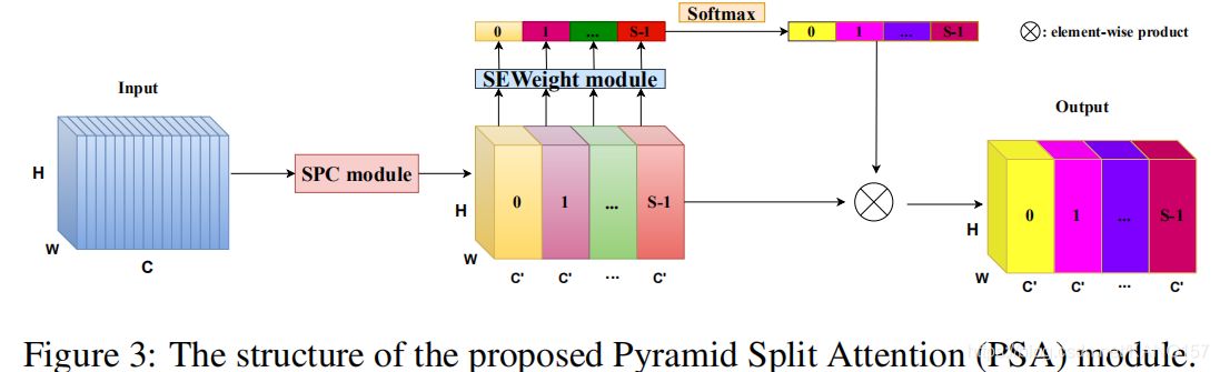
**5.金字塔特征注意力网络(Pyramid FeatureAttention Network(2019CVPR)**SE仅仅考虑了通道注意力,忽略了空间注意力。2.BAM和CBAM考虑了通道注意力和空间注意力,但仍存在两个最重要的缺点:(1)没有捕获不同尺度的空间信息来丰富特征空间。(2)空间注意力仅仅考虑了局部区域的信息,而无法建立远距离的依赖。3.后续出现的PyConv,Res2Net和HS-ResNet都用于解决CBAM的这两个缺点,但计算量太大。
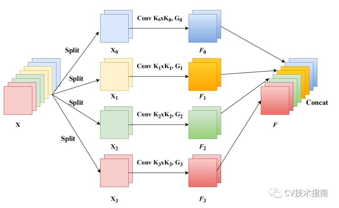
PSA模块
- 代码实现
class SEWeightModule(nn.Module): def __init__(self, channels=64, reduction=16): super(SEWeightModule, self).__init__() self.avg_pool = nn.AdaptiveAvgPool2d(1) self.fc1 = nn.Conv2d(channels, channels // reduction, kernel_size=1, stride=1, padding=0) self.relu = nn.ReLU(inplace=True) self.fc2 = nn.Conv2d(channels // reduction, channels, kernel_size=1, stride=1, padding=0) self.sigmoid = nn.Sigmoid() def forward(self, x): x = self.avg_pool(x) x = self.fc1(x) x = self.relu(x) x = self.fc2(x) x = self.sigmoid(x) return xclass PAM_Module(nn.Module): # Position attention module def __init__(self, in_dim=64): super(PAM_Module, self).__init__() self.chanel_in = in_dim self.query_conv = nn.Conv2d(in_channels=in_dim, out_channels=in_dim // 2, kernel_size=1) self.key_conv = nn.Conv2d(in_channels=in_dim, out_channels=in_dim // 2, kernel_size=1) self.value_conv = nn.Conv2d(in_channels=in_dim, out_channels=in_dim, kernel_size=1) self.gamma = nn.Parameter(torch.zeros(1)) self.softmax = nn.Softmax(dim=-1) def forward(self, x): # inputs : # x : input feature maps( B, C, H, W) # returns : # out : attention value + input feature # attention: B*(H*W)*(H*W) # [105, 16, 19, 19] m_batchsize, C, height, width = x.size() proj_query = self.query_conv(x).view(m_batchsize, -1, width * height).permute(0, 2, 1) proj_key = self.key_conv(x).view(m_batchsize, -1, width * height) energy = torch.bmm(proj_query, proj_key) attention = self.softmax(energy) proj_value = self.value_conv(x).view(m_batchsize, -1, width * height) out = torch.bmm(proj_value, attention.permute(0, 2, 1)) out = out.view(m_batchsize, C, height, width) out = self.gamma * out + x return out# 通道注意力class CAM_Scale(nn.Module): def __init__(self , channels=64 , ratio = 16): super(CAM_Scale, self).__init__() self.avg_pool = nn.AdaptiveAvgPool2d(1) # 通道数不变,H*W*C变为1*1*64 self.max_pool = nn.AdaptiveMaxPool2d(1) self.fc_layers=nn.Sequential( nn.Conv2d(channels , channels // ratio , 1 , bias = False), nn.LeakyReLU(), nn.Conv2d(channels//ratio , channels ,1, bias = False) ) self.sigmoid = nn.Sigmoid() def forward(self , x): avg_out = self.fc2(self.leakyrelu(self.fc1(self.avg_pool(x)))) #两层神经网络共享 max_out = self.fc2(self.leakyrelu(self.fc1(self.max_pool(x)))) out = self.sigmoid(avg_out + max_out) return x*outclass DANetHead(nn.Module): def __init__(self, in_channels=64, out_channels=64): super(DANetHead, self).__init__() inter_channels = in_channels // 4 self.conv5a = nn.Sequential( nn.Conv2d(in_channels, inter_channels, 3, padding=1, bias=False), nn.BatchNorm2d(inter_channels), nn.LeakyReLU()) self.conv5c = nn.Sequential( nn.Conv2d(in_channels, inter_channels, 3, padding=1, bias=False), nn.BatchNorm2d(inter_channels), nn.leakyReLU()) self.sa = PAM_Module(inter_channels) self.sc = CAM_Module(inter_channels) self.conv51 = nn.Sequential( nn.Conv2d(inter_channels, inter_channels, 3, padding=1, bias=False), nn.BatchNorm2d(inter_channels), nn.LeakyReLU()) self.conv52 = nn.Sequential( nn.Conv2d(inter_channels, inter_channels, 3, padding=1, bias=False), nn.BatchNorm2d(inter_channels), nn.LeakyReLU()) self.conv8 = nn.Sequential(nn.Dropout2d(0.1, False), nn.Conv2d(inter_channels, out_channels, 1)) # se self.se = SEWeightModule(out_channels) def forward(self, x): feat1 = self.conv5a(x) sa_feat = self.sa(feat1) sa_conv = self.conv51(sa_feat) feat2 = self.conv5c(x) sc_feat = self.sc(feat2) sc_conv = self.conv52(sc_feat) feat_sum = sa_conv + sc_conv sasc_output = self.conv8(feat_sum) # se sasc_output = self.se(sasc_output) return sasc_output# Pyramid Split Dual Attentionclass PSDAModule(nn.Module): def __init__(self, inplans=64, planes=64, conv_kernels=[3, 5, 7, 9], stride=1, conv_groups=[1, 4, 8, 16]): super(PSDAModule, self).__init__() self.conv_1 = nn.Conv2d(inplans, planes // 4, kernel_size=conv_kernels[0], padding=conv_kernels[0] // 2, stride=stride, groups=conv_groups[0]) self.conv_2 = nn.Conv2d(inplans, planes // 4, kernel_size=conv_kernels[1], padding=conv_kernels[1] // 2, stride=stride, groups=conv_groups[1]) self.conv_3 = nn.Conv2d(inplans, planes // 4, kernel_size=conv_kernels[2], padding=conv_kernels[2] // 2, stride=stride, groups=conv_groups[2]) self.conv_4 = nn.Conv2d(inplans, planes // 4, kernel_size=conv_kernels[3], padding=conv_kernels[3] // 2, stride=stride, groups=conv_groups[3]) self.dan = DANetHead(planes // 4, planes // 4) self.split_channel = planes // 4 self.softmax = nn.Softmax(dim=1) def forward(self, x): batch_size = x.shape[0] # 多尺度分组 x1 = self.conv_1(x) x2 = self.conv_2(x) x3 = self.conv_3(x) x4 = self.conv_4(x) feats = torch.cat((x1, x2, x3, x4), dim=1) # [105, 64, 41, 41] feats = feats.view(batch_size, 4, self.split_channel, feats.shape[2], feats.shape[3]) # [105, 4, 16, 41, 41] x1_dan = self.dan(x1) # [105, 16, 1, 1] x2_dan = self.dan(x2) x3_dan = self.dan(x3) x4_dan = self.dan(x4) x_se = torch.cat((x1_dan, x2_dan, x3_dan, x4_dan), dim=1) # [105, 64, 1, 1] attention_vectors = x_se.view(batch_size, 4, self.split_channel, 1, 1) attention_vectors = self.softmax(attention_vectors) feats_weight = feats * attention_vectors for i in range(4): x_se_weight_fp = feats_weight[:, i, :, :] if i == 0: out = x_se_weight_fp else: out = torch.cat((x_se_weight_fp, out), dim=1) return out
版权归原作者 一个菜鸟的成长史 所有, 如有侵权,请联系我们删除。