

本期文章分为两期,第一篇我们先解决是否Steam平台的游戏会不会打折?下一期我们会详细分析影响Steam的打折因素

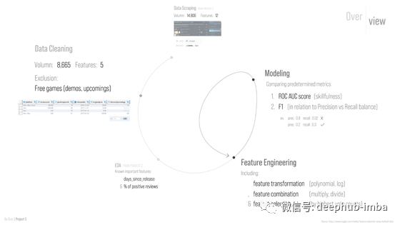
基本目标
使用有监督的机器学习分类模型来确定某款Steam游戏是否可以在正常一周内(没有大规模的折扣事件)出现折扣。
数据
在Steam官网上获得的数据。
为了更容易访问,我们将收集的数据集上传到我的AWS实例中。为了访问数据,我们将使用外部Python软件包SQLAlchemy和独立的数据库工具DBeaver来与AWS服务器通信,以检查和清理数据。最后,数据库在PostgreSQL中处理完毕。
您可以找到我用来从Jupyter Notebook中加载此项目的数据的代码。

数据清洗
因为原始数据集包含许多空值,以及不同的大小写,例如('Free'与'free')。以下SQL语句将缩小范围,并在此过程中创建自定义视图“cleaned_raw”:
create view cleaned_raw as
select * from steam_3t_strat sts
where title isnotnull
and reviewcount isnotnull
and originalprice isnotnull
and afterdiscount isnotnull
and originalprice notlike'%ree%'
and originalprice like'%.%'
现在我们已经去掉了一些空条目,现在我们对每一列进行格式化,使每一列的数据类型(int、float、string、datetime等)符合本身的含义:
deletefrom cleaned_raw where releasedate isnull

create view baseline as
  select platform, reviewcount, positivepercent , releasedate::date,
          cast(originalprice asdoubleprecision) , discountpercentage , alltags
  from cleaned_raw;
准备好分析数据之前的最后几个步骤将包含一些基本的特征工程:
- 将列“platform” 二值化为“multi platform” (也即这一款游戏是否在多平台上发售);
- 在原始的“discount percentage”列基础上创建一个模型需要预测的目标列,其含义为0代表没有打折,1代表打折。
- 最后,从上一个项目中,我们知道“days_since_release”(游戏发售多久了)是最重要的特性之一,因此我们将从“release date”列进行特征工程,但这次是用SQL完成的。
现在,有了新视图“basic_fe”,我们就可以在Jupyter Notebook中进行特征工程与模型构建。
探索性数据分析
由于这是我上一个项目的延续,大部分的EDA都已经完成了,这里我们将直接进入特征工程。
定义评价指标
对于这个项目,模型能够同时达到有效与平衡。因此,我将主要研究两个指标:
- ROC-AUC评分(模型有效性)
- F1分数(查准率和查全率之间的调和平均值)
注:我也会看查准率和查全率的平衡,例如,如果查准率是0.8,查全率是0.02,这对我来说太不平衡了,所以即使它产生了一个整体更好的F1分数,我也不会采取这种模式。
建立基线模型
现在我们进入该项目最有趣的部分,但首先我们导入在AWS进行数据清洗后的特征并建立基线模型,以便我们可以将其与将来的模型进行比较。
basic_fe = pd.read_sql_query('''SELECT * FROM basic_fe''', cnx)

在我们进一步讨论之前,让我们先来观察一下类别不平衡性:
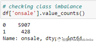
类别不平衡非常严重,但我们可以对少数类计算类别权重,用于分类模型的构建:

现在,在删除一些不需要的观察值和列之后,运行模型:
# copy the feature engineered view for exploratory purposes
df = basic_fe.copy()
# dropping unneeded columns
df.drop(['platform', 'releasedate', 'alltags', 'discountpercentage'], axis=1, inplace = True)
# cleaning NaN values
df.fillna(0, inplace=True)

# splitting data and target
X, y = df.drop('onsale',axis=1), df['onsale']

# run baseline models (train-test split is conducted within this function)
baseline_model = classification(X, y, {0: 1, 1: 15})
请注意,我正在运行的
classification()
函数是一个自定义函数,包含7种模型,其中包括:
- 最近邻分类器(n_neighbors=5)
- 逻辑回归(C=0.95)
- 高斯型朴素贝叶斯分类器
- 支持向量机(gamma=’auto’,probability=True)
- 决策树(random_state=5)*
- 随机森林(random_state=5)
- 梯度提升机(n_estimators = 90, max_depth = 100)
classification()
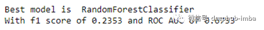
函数将对每个模型打印AUC值与ROC曲线。它还将自动确定并返回七个模型中评估指标最高的模型以及特征重要性分数。在这种情况下,对于基线模型:
特征工程
由于该项目的重点是利用手头的可用数据获得最佳模型,因此我们将不得不在迭代过程中尝试使用不同的特征工程方法。
以下是我在此项目中使用的三种有效方法,尽管过程绝对不那么顺利。
总结一下我的过程,整体流程如下:

1. 特征变换
首先,让我们用从StackOverflow获得的一个很有用的函数对特征进行多项式变换:
defPolynomialFeatures_labeled(input_df,power):
    '''
    Basically this is a cover for the sklearn preprocessing function.
    The problem with that function is if you give it a labeled dataframe, it ouputs an unlabeled dataframe with potentially
    a whole bunch of unlabeled columns.
    Inputs:
    input_df = Your labeled pandas dataframe (list of x's not raised to any power)
    power = what order polynomial you want variables up to. (use the same power as you want entered into pp.PolynomialFeatures(power) directly)
    Output:
    Output: This function relies on the powers_ matrix which is one of the preprocessing function's outputs to create logical labels and
    outputs a labeled pandas dataframe
    '''
    poly = PolynomialFeatures(power)
    output_nparray = poly.fit_transform(input_df)
    powers_nparray = poly.powers_

    input_feature_names = list(input_df.columns)
    target_feature_names = ["Constant Term"]
    forfeature_distillationinpowers_nparray[1:]:
        intermediary_label = ""
        final_label = ""
        foriinrange(len(input_feature_names)):
            iffeature_distillation[i] == 0:
                continue
            else:
                variable = input_feature_names[i]
                power = feature_distillation[i]
                intermediary_label = "%s^%d"% (variable,power)
                iffinal_label == "":         #If the final label isn't yet specified
                    final_label = intermediary_label
                else:
                    final_label = final_label+" x "+intermediary_label
        target_feature_names.append(final_label)
    output_df = pd.DataFrame(output_nparray, columns = target_feature_names)
    returnoutput_df
构建模型并返回分类评价指标:
# poly transform the data
explore_X_poly=PolynomialFeatures_labeled(X,2)

# run modeling to see metrics
classification(explore_X_poly, y, {0: 1, 1: 15})
可以看到相比基线模型我们的结果还稍微变差了一些,看来多项式变换无法完成这一分类任务,下面我们换另一种方法:
2. 特征结合
我编写了一个自定义算法来探索不同的特征组合,看这样做是否可以提高模型分数:
defexplore_fe(df, target):
    '''
    A function to do exploratory feature engineering.
    It's flexible in its purpose, and is currently configured for this project only.
    Inputs:
    df (like X) = Your dataset without the target (y)
    target (like y) = Your target, whatever you are trying to predict ---Binary.
    Output:
    Returns engineered X (dataframe without target) based on the engineering logic.
    '''
    df = df.astype(float)
    df = df.replace({0:1 , 1:2})

    foriinrange (0, len(df.columns)):
        df[f'{df.columns[i]}^2'] = np.square(df[df.columns[i]])
        df[f'{df.columns[i]}^1/2'] = np.sqrt(df[df.columns[i]])
        df[f'{df.columns[i]} * {df.columns[i+1]}'] = df[df.columns[i]] *df[df.columns[i+1]]
        df[f'{df.columns[i]} / {df.columns[i+1]}'] = df[df.columns[i]] /df[df.columns[i+1]]
#         df[f'{df.columns[i]} + {df.columns[i+1]}'] = df[df.columns[i]] + df[df.columns[i+1]]
#         df[f'{df.columns[i]} - {df.columns[i+1]}'] = df[df.columns[i]] - df[df.columns[i+1]]


#     df.fillna(0, inplace = True)
#     df.replace([np.inf, -np.inf], np.nan).dropna(axis=1)
    df[~df.isin([np.nan, np.inf, -np.inf]).any(1)].astype(np.float64)

    X,y= df, target
    X_train, X_test, y_train, y_test = train_test_split(X, y, test_size = 0.3, random_state=4444)

    ran = RandomForestClassifier(random_state=5)
    ran.fit(X_train, y_train)

    print ('Accuracy: ', accuracy_score(y_test, ran.predict(X_test)))
    print("Precision: {:6.4f},   Recall: {:6.4f},   f1: {:6.4f}".format(precision_score(y_test, ran.predict(X_test)),
                                                 recall_score(y_test, ran.predict(X_test)), f1_score(y_test, ran.predict(X_test))), '\n')

    k = list(X.columns)
    pp = pprint.PrettyPrinter(indent=4)
    pp.pprint(sorted(list(zip(k, ran.feature_importances_)), key=lambdax: x[1], reverse=True))

    returndf
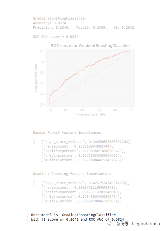
这一函数基本就是对所有特征逐列进行特征的乘除操作以非线性组合出新特征。处理完毕后我们再次运行模型并且获得了以下结果:
3. 特征选择
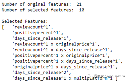
从最后两个步骤开始,我现在有了一个包含21组特征的的数据集,其中16组特征都是经过特征工程获得的,这可能会导致过拟合,并且“噪声”水平可能过高。因此,我们对特征进行了特征选择:
deffeature_selection(X, y, score_to_keep = 5):
    '''
    A function to select features by votes of 6 models who can calculate feature importances.
    Also prints out how many original features there are, how many selected, and a list of selected features.
    Original idea from https://www.kaggle.com/mlwhiz/feature-selection-using-football-data
    Inputs:
    X = Your dataset without the target (y)
    y = Your target, whatever you are trying to predict --- Binary.
    score_to_keep = Pick features that have a 'score_to_keep' amount of votes --- max is 6 votes, default is 5.

    Output:
    Returns selected_X as a dataframe without target(y).
    '''
    feature_name = list(X.columns)
    num_feats=len(X.columns)
    defcor_selector(X, y,num_feats):
        cor_list = []
        feature_name = X.columns.tolist()
        # calculate the correlation with y for each feature
        foriinX.columns.tolist():
            cor = np.corrcoef(X[i], y)[0, 1]
            cor_list.append(cor)
        # replace NaN with 0
        cor_list = [0ifnp.isnan(i) elseiforiincor_list]
        # feature name
        cor_feature = X.iloc[:,np.argsort(np.abs(cor_list))[-num_feats:]].columns.tolist()
        # feature selection? 0 for not select, 1 for select
        cor_support = [Trueifiincor_featureelseFalseforiinfeature_name]
        returncor_support, cor_feature
    cor_support, cor_feature = cor_selector(X, y,num_feats)

    X_norm = MinMaxScaler().fit_transform(X)
    chi_selector = SelectKBest(chi2, k=num_feats)
    chi_selector.fit(X_norm, y)
    chi_support = chi_selector.get_support()
    chi_feature = X.loc[:,chi_support].columns.tolist()

    rfe_selector = RFE(estimator=LogisticRegression(), n_features_to_select=num_feats, step=10, verbose=5)
    rfe_selector.fit(X_norm, y)
    rfe_support = rfe_selector.get_support()
    rfe_feature = X.loc[:,rfe_support].columns.tolist()

    embeded_lr_selector = SelectFromModel(LogisticRegression(penalty="l2"), max_features=num_feats)
    embeded_lr_selector.fit(X_norm, y)
    embeded_lr_support = embeded_lr_selector.get_support()
    embeded_lr_feature = X.loc[:,embeded_lr_support].columns.tolist()

    embeded_rf_selector = SelectFromModel(RandomForestClassifier(n_estimators=100), max_features=num_feats)
    embeded_rf_selector.fit(X_norm, y)
    embeded_rf_support = embeded_rf_selector.get_support()
    embeded_rf_feature = X.loc[:,embeded_rf_support].columns.tolist()

    lgbc=LGBMClassifier(n_estimators=500, learning_rate=0.05, num_leaves=32, colsample_bytree=0.2,
            reg_alpha=3, reg_lambda=1, min_split_gain=0.01, min_child_weight=40)
    embeded_lgb_selector = SelectFromModel(lgbc, max_features=num_feats)
    embeded_lgb_selector.fit(X_norm, y)
    embeded_lgb_support = embeded_lgb_selector.get_support()
    embeded_lgb_feature = X.loc[:,embeded_lgb_support].columns.tolist()

    feature_selection_df = pd.DataFrame({'Feature':feature_name, 'Pearson':cor_support, 'Chi-2':chi_support, 'RFE':rfe_support, 'Logistics':embeded_lr_support,
                                        'Random Forest':embeded_rf_support, 'LightGBM':embeded_lgb_support})

    feature_selection_df['Total'] = np.sum(feature_selection_df, axis=1)

    feature_selection_df = feature_selection_df.sort_values(['Total','Feature'] , ascending=False)
    feature_selection_df.index = range(1, len(feature_selection_df)+1)


    selected_X = X.copy()
    to_drop = []
    foriinrange (0, len(feature_selection_df)):
        iffeature_selection_df.Total.values[i] <score_to_keep:
            to_drop.append(feature_selection_df.Feature.values[i])

    selected_X = selected_X.drop(to_drop, axis = 1)

    print ("Number of orginal features: ", num_feats)
    print ("Number of selected features: ", len(selected_X.columns), '\n')
    pp = pprint.PrettyPrinter(indent=4)
    print("Selected Features:")
    pp.pprint(list(selected_X.columns))


    returnselected_X
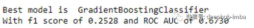
结合步骤1和2,然后根据投票数选择有效特征,以下为运行结果:

我们最终制作了一个比基线模型稍好的模型。我对这个基于有限数据的模型很满意,但我们还并没有完成,让我们试着通过调整阈值使它变得更好。
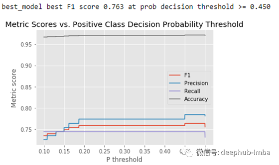
阈值调整
阈值调整不仅仅是建模的最后一步,这对模型的表现也至关重要,因为调整查准率与查全率之间的平衡——也即阈值——直接影响最后评估指标。
我们将使用以下代码检查最佳阈值:
# Splitting the data again to make sure we are using the dataset that was fed into the best model
X, y  = exp_Xpoly_sel_5, y
X_train, X_test, y_train, y_test = train_test_split(X, y, test_size = 0.2, random_state=42)
X_val, y_val = X_test, y_test# explicitly calling this validation since we're using it for selection

thresh_ps = np.linspace(.10,.50,1000)
model_val_probs = best_model.predict_proba(X_val)[:,1] # positive class probs, same basic logistic model we fit in section 2

f1_scores, prec_scores, rec_scores, acc_scores = [], [], [], []
forpinthresh_ps:
    model_val_labels = model_val_probs>= p
    f1_scores.append(f1_score(y_val, model_val_labels))
    prec_scores.append(precision_score(y_val, model_val_labels))
    rec_scores.append(recall_score(y_val, model_val_labels))
    acc_scores.append(accuracy_score(y_val, model_val_labels))

plt.plot(thresh_ps, f1_scores)
plt.plot(thresh_ps, prec_scores)
plt.plot(thresh_ps, rec_scores)
plt.plot(thresh_ps, acc_scores)

plt.title('Metric Scores vs. Positive Class Decision Probability Threshold')
plt.legend(['F1','Precision','Recall','Accuracy'])
plt.xlabel('P threshold')
plt.ylabel('Metric score')

best_f1_score = np.max(f1_scores)
best_thresh_p = thresh_ps[np.argmax(f1_scores)]

print('best_model best F1 score %.3f at prob decision threshold >= %.3f'
      % (best_f1_score, best_thresh_p))
结论
现在我们有了阈值为0.45,ROC-AUC分数为0.7097的最佳模型。
既然我们已经建立了这个模型,那么为什么不用呢?所以我创建了一个把我先前的项目与这个项目结合在一起的应用程序。
作者:Da Guo
deephub翻译组:Alexander Zhao
本文代码会和下期文章一起发布
DeepHub
微信号 : deephub-imba
每日大数据和人工智能的重磅干货
大厂职位内推信息
长按识别二维码关注 ->
好看就点在看!********** **********