OPENCV图像直方图以及均值化

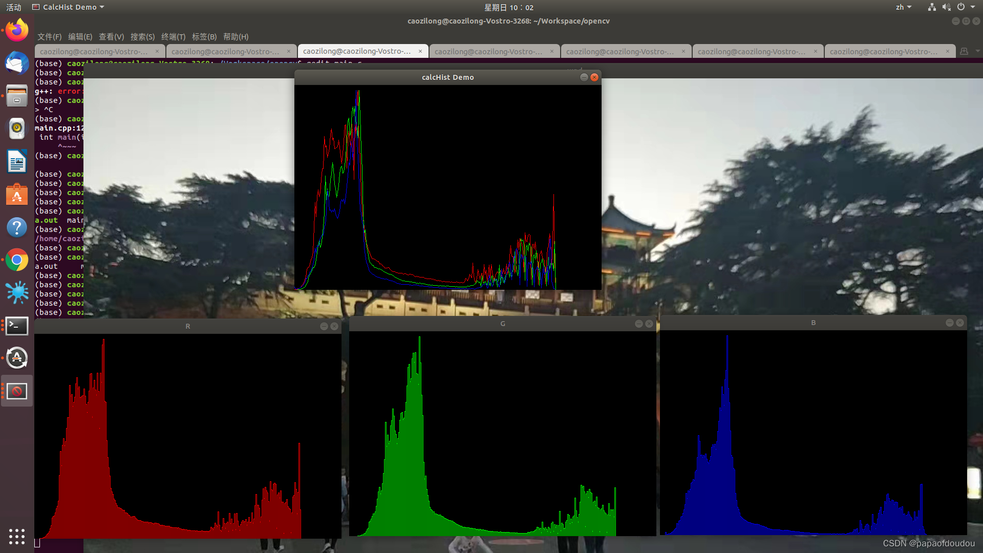
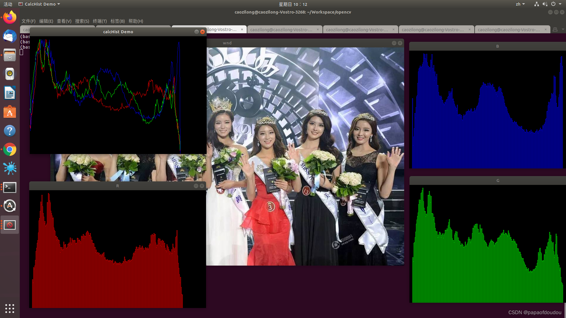
直方图是我们在照片中使用来查看图像中每个值有多少像素，照片中的每个像素的值都从0(黑色)到255(白色)，图的左侧代表音阶的暗色调，右侧代表较亮的色调。在彩色摄影中，每个像素对于每种颜色都有其自己的值(0-255)。图片中的直方图显示了每种颜色(红色，蓝色和绿色)的像素值分布.

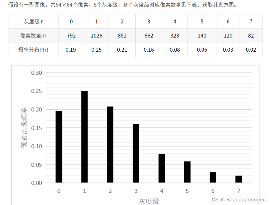
图像直方图，也叫灰度直方图，反映了图像像素分布的统计特征，是图像处理中简单有效的工具，图像直方图广泛地应用于图像处理的各个领域，如：特征提取，图像匹配，灰度图像的阈值分割，基于颜色的图像检索以及图像分类。

图像的直方图的形态很大程度上可直观的反映图像的质量情况，比如根据下图所示，会很快发现一张图片是否过量还是过暗。

图像直方图的优点是，计算量较小，且具有图像平移，旋转，缩放不变性等。

数学原理

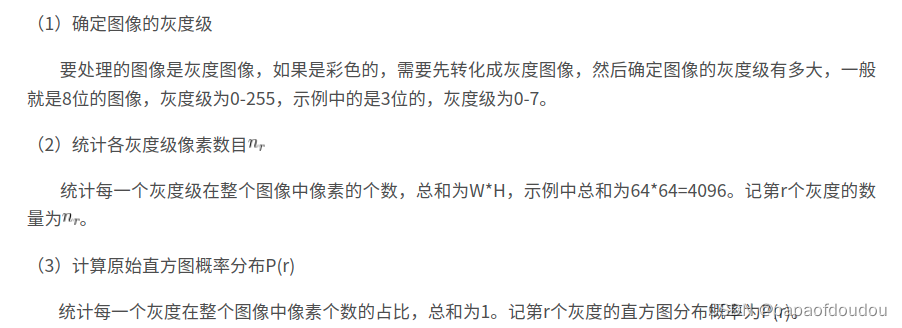
图像灰度直方图计算：

其中，W，H分别表示图像的宽和高，表示图像中像素值为r的数量,表示图像中像素值为r的比率，L是指图像灰度级数，比如，8BIT的灰度图像L=2^8=256.其存在256个色阶，即0-255。

OPENCV获取直方图：

//获得直方图
#include <opencv2/core/core.hpp>
#include <opencv2/highgui/highgui.hpp>
#include <opencv2/imgproc/imgproc.hpp>
#include <iostream>
using namespace cv;
using namespace std;
int main(int argc, char** argv)
{
    //----------------------example 1-------------------------------//
    Mat src, dst;
    /// Load image
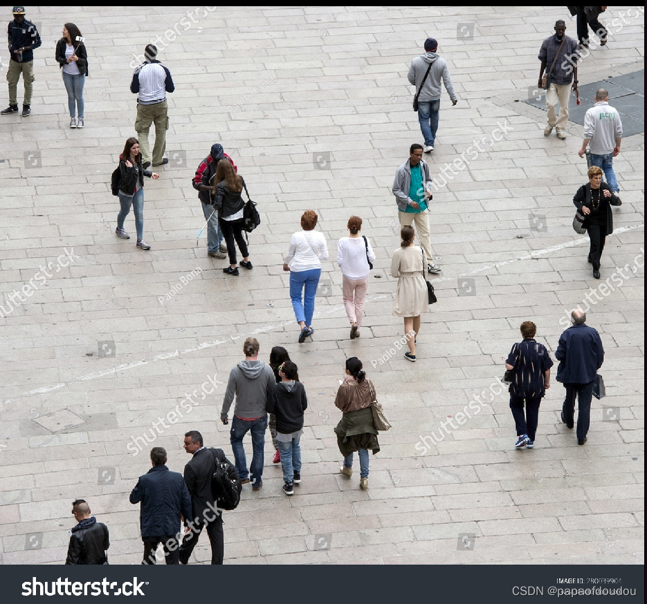
    src = imread("/home/caozilong/165823915.jpg");
    if (!src.data)
    {
        cout << "load image failed" << endl;
        return -1;
    }
    /// Separate the image in 3 places ( R, G and B )
    vector<Mat> rgb_planes;
    Mat hsv;
    cvtColor(src, hsv, COLOR_BGR2HSV);
    split(hsv, rgb_planes);
    split(src, rgb_planes);
    /// Establish the number of bins 
    int histSize = 256;
    /// Set the ranges ( for R,G,B) )
    float range[] = { 0, 255 };
    const float* histRange = { range };
    bool uniform = true; bool accumulate = false;
    Mat r_hist, g_hist, b_hist;
    /// Compute the histograms:
    calcHist(&rgb_planes[2], 1, 0, Mat(), r_hist, 1, &histSize, &histRange, uniform, accumulate);
    calcHist(&rgb_planes[1], 1, 0, Mat(), g_hist, 1, &histSize, &histRange, uniform, accumulate);
    calcHist(&rgb_planes[0], 1, 0, Mat(), b_hist, 1, &histSize, &histRange, uniform, accumulate);
    // Draw the histograms for R, G and B
    int hist_w = 600; int hist_h = 400;
    int bin_w = cvRound((double)hist_w / histSize);
    Mat rgb_hist[3];
    for (int i = 0; i < 3; ++i)
    {
        rgb_hist[i] = Mat(hist_h, hist_w, CV_8UC3, Scalar::all(0));
    }
    Mat histImage(hist_h, hist_w, CV_8UC3, Scalar(0, 0, 0));
    /// Normalize the result to [ 0, histImage.rows-10]
    normalize(r_hist, r_hist, 0, histImage.rows - 10, NORM_MINMAX);
    normalize(g_hist, g_hist, 0, histImage.rows - 10, NORM_MINMAX);
    normalize(b_hist, b_hist, 0, histImage.rows - 10, NORM_MINMAX);
    /// Draw for each channel 
    for (int i = 1; i < histSize; i++)
    {
        line(histImage, Point(bin_w * (i - 1), hist_h - cvRound(r_hist.at<float>(i - 1))),
            Point(bin_w * (i), hist_h - cvRound(r_hist.at<float>(i))),
            Scalar(0, 0, 255), 1);
        line(histImage, Point(bin_w * (i - 1), hist_h - cvRound(g_hist.at<float>(i - 1))),
            Point(bin_w * (i), hist_h - cvRound(g_hist.at<float>(i))),
            Scalar(0, 255, 0), 1);
        line(histImage, Point(bin_w * (i - 1), hist_h - cvRound(b_hist.at<float>(i - 1))),
            Point(bin_w * (i), hist_h - cvRound(b_hist.at<float>(i))),
            Scalar(255, 0, 0), 1);
    }
    for (int j = 0; j < histSize; ++j)
    {
        int val = saturate_cast<int>(r_hist.at<float>(j));
        rectangle(rgb_hist[0], Point(j * 2 + 10, rgb_hist[0].rows), Point((j + 1) * 2 + 10, rgb_hist[0].rows - val), Scalar(0, 0, 255), 1, 8);
        val = saturate_cast<int>(g_hist.at<float>(j));
        rectangle(rgb_hist[1], Point(j * 2 + 10, rgb_hist[1].rows), Point((j + 1) * 2 + 10, rgb_hist[1].rows - val), Scalar(0, 255, 0), 1, 8);
        val = saturate_cast<int>(b_hist.at<float>(j));
        rectangle(rgb_hist[2], Point(j * 2 + 10, rgb_hist[2].rows), Point((j + 1) * 2 + 10, rgb_hist[2].rows - val), Scalar(255, 0, 0), 1, 8);
    }
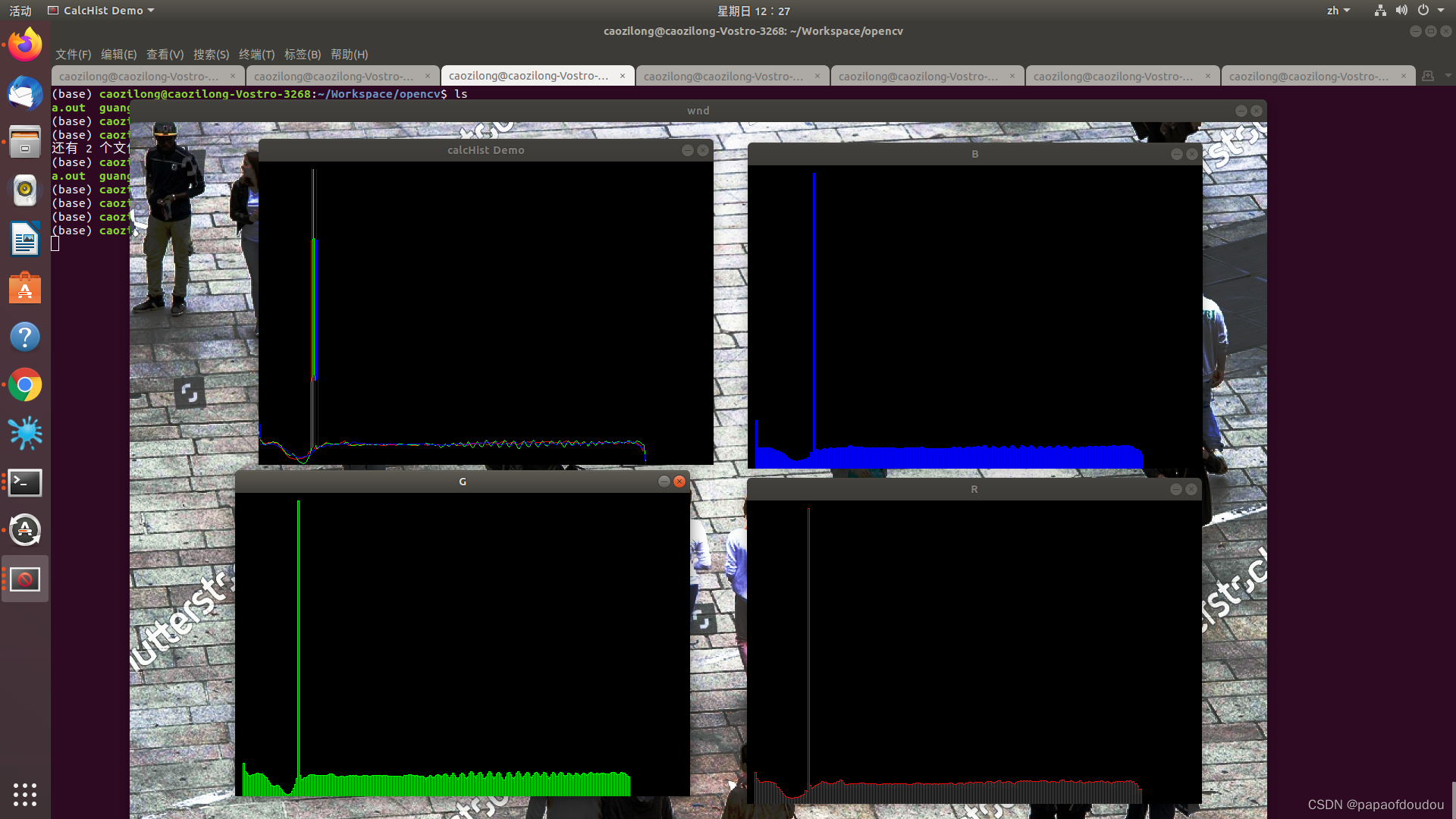
    /// Display 
    namedWindow("calcHist Demo", CV_WINDOW_AUTOSIZE);
    namedWindow("wnd");
    imshow("calcHist Demo", histImage);
    imshow("wnd", src);
    imshow("R", rgb_hist[0]);
    imshow("G", rgb_hist[1]);
    imshow("B", rgb_hist[2]);
    waitKey();
}

g++ new.cpp `pkg-config --cflags --libs opencv`

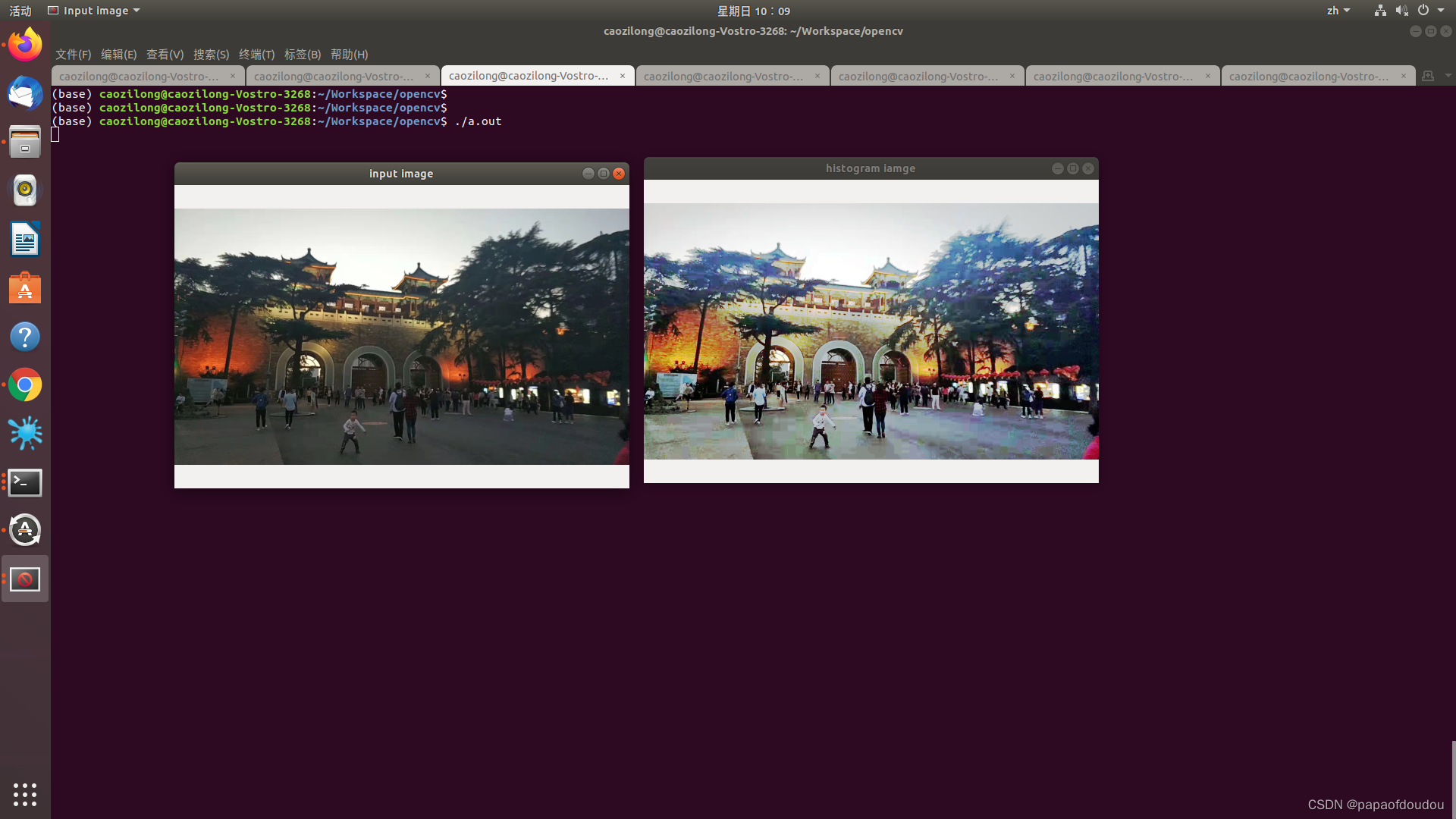
直方图均值化

直方图均衡化是通过拉伸像素强度的分布范围，使得在0~255灰阶上的分布更加均衡，提高了图像的对比度，达到改善图像主观视觉效果的目的。对比度较低的图像适合使用直方图均衡化方法来增强图像细节。

//彩色图像直方图均衡化
#include<opencv2/opencv.hpp>
#include<iostream>
#include<cmath>
using namespace cv;
using namespace std;
const char* output = "histogram iamge";
int main(int argc, char** argv)
{
    Mat src, dst, dst1;
    src = imread("/home/caozilong/165823915.jpg");
    if (!src.data)
    {
        printf("could not load image...\n");
        return -1;
    }
    char input[] = "input image";
    namedWindow(input, 0);
    namedWindow(output, 0);
    resizeWindow(input, 600, 400);
    imshow(input, src);
    //分割通道
    vector<Mat>channels;
    split(src, channels);
    Mat blue, green, red;
    blue = channels.at(0);
    green = channels.at(1);
    red = channels.at(2);
    //分别对BGR通道做直方图均衡化
    equalizeHist(blue, blue);
    equalizeHist(green, green);
    equalizeHist(red, red);
    //合并通道
    merge(channels, dst);
    resizeWindow(output, 600, 400);
    imshow(output, dst);
    waitKey(0);
    return 0;
}

g++ main.cpp `pkg-config --cflags --libs opencv`

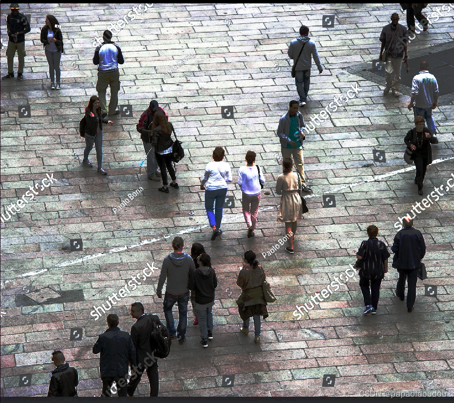
可以看到对比度确实增加了

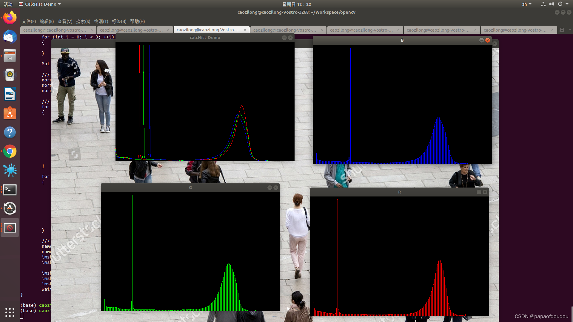
但是对于那些曝光良好，直方图表现均匀的图像，均值化的效果并不明显：

然后，进行均值化后的效果，可以发现，对比度的增加效果并不明显：

另一个例子，原始图片：

图像直方图：

进行直方图均值化后的图像：

对应的直方图为：

结束！