
1 概述
在许多问题中,可能既包含着纯线性函数,也包含着分段线性函数。在这一节,我们使用运输问题解释处理分段线性模型的各种方法。
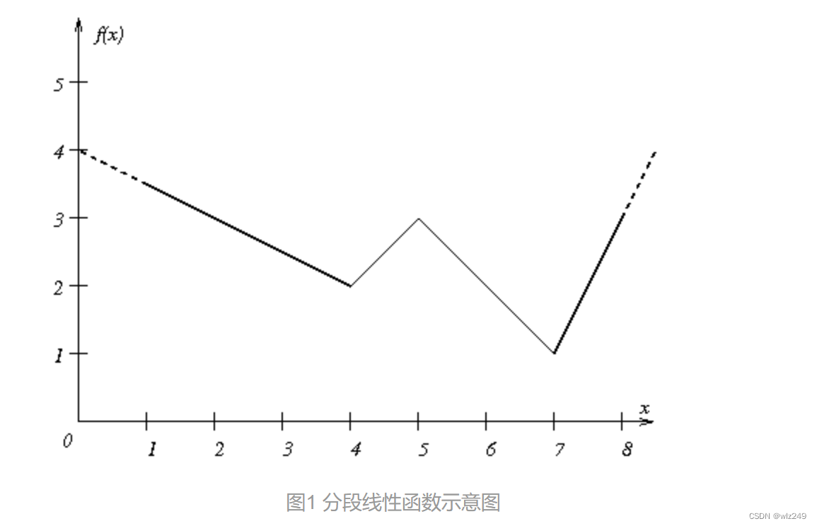
从几何的观点,下图为一个经典的分段线性函数。这个函数由四条线段构成,分段点为4、5 和 7。这三个分段点,将整个函数分为(-∞, 4) 、 [4, 5) 、 [5, 7) 和 [7, ∞) 四个区间。
每个区间内线段的斜率是一个常数,但不同区间之间的线段斜率是不同的。斜率的变化的点就是分段点。
分段线性函数常用于表示或逼近非线性一元函数。
2 算例及Python|Gurobi实现
2.1 算例
考虑经典的运输问题,即:有一些供应商(节点i)和一些需求(节点j),确定每个供应商的产量() 、用户的需求量(
) ,以及在给定每条路径运输成本
的情况下,最小化运输成本。
2.2 Python|Gurobi实现
# -*- coding: utf-8 -*-

from gurobipy import *
import numpy as np

N_i=3
N_j=4
k=1.8

C=np.array([
    [0.0755,0.0655,0.0498,0.0585],
    [0.0276,0.0163,0.0960,0.0224],
    [0.0680,0.0119,0.0340,0.0751]
    ])

Pmin=np.array([100,50,30])
Pmax=np.array([450,350,500])
demand=np.array([217,150,145,244])

# 创建模型
M_PWL=Model("PWL-1")

# 变量声明
x  =M_PWL.addVars(N_i,N_j,lb=0,ub=100, name="x")
P  =M_PWL.addVars(N_i,lb=0,ub=Pmax, name="P")
U  =M_PWL.addVars(N_i,vtype=GRB.BINARY,name="U")  #采用0-1变量对分段约束进行线性化处理。即:通过定义0-1变量“U”,

# 设置目标函数
M_PWL.setObjective(quicksum(C[i,j]*x[i,j]*x[i,j] for i in range(N_i) for j in range(N_j)),GRB.MINIMIZE)

# 添加约束
M_PWL.addConstrs((P[i]<=Pmax[i]*U[i] for i in range(N_i)),"Con_P1")
M_PWL.addConstrs((P[i]>=Pmin[i]*U[i] for i in range(N_i)),"Con_P2")

M_PWL.addConstrs((sum(x[i,j] for i in range(N_i))>=demand[j] for j in range(N_j)),"Con_x1")
M_PWL.addConstrs((sum(x[i,j] for j in range(N_j))==P[i] for i in range(N_i)),"Con_x2")

# Optimize model
M_PWL.optimize()

M_PWL.write("PWL1.lp")

P_c=np.zeros(N_i)
x_c=np.zeros((N_i,N_j))

for i in range(N_i):
    P_c[i]=P[i].x
    for j in range(N_j):
        x_c[i,j]=x[i,j].x

print('P_c is',P_c)
print('x_c is',x_c)
2.3 运行结果
Gurobi Optimizer version 9.5.2 build v9.5.2rc0 (win64)
Thread count: 8 physical cores, 16 logical processors, using up to 16 threads
Optimize a model with 13 rows, 18 columns and 39 nonzeros
Model fingerprint: 0xc29ac6cf
Model has 12 quadratic objective terms
Variable types: 15 continuous, 3 integer (3 binary)
Coefficient statistics:
  Matrix range     [1e+00, 5e+02]
  Objective range  [0e+00, 0e+00]
  QObjective range [2e-02, 2e-01]
  Bounds range     [1e+00, 5e+02]
  RHS range        [1e+02, 2e+02]
Presolve removed 7 rows and 6 columns
Presolve time: 0.00s
Presolved: 6 rows, 12 columns, 20 nonzeros
Presolved model has 12 quadratic objective terms
Variable types: 12 continuous, 0 integer (0 binary)
Root relaxation presolve time: 0.00s
Root relaxation presolved: 6 rows, 12 columns, 20 nonzeros
Root relaxation presolved model has 12 quadratic objective terms
Root barrier log...

Ordering time: 0.00s

Barrier statistics:
 AA' NZ     : 8.000e+00
 Factor NZ  : 2.100e+01
 Factor Ops : 9.100e+01 (less than 1 second per iteration)
 Threads    : 1

                  Objective                Residual
Iter       Primal          Dual         Primal    Dual     Compl     Time
   0   3.49914954e+06 -3.87161263e+06  3.49e+03 8.83e+02  1.01e+06     0s
   1   1.27698128e+05 -5.62657044e+05  3.70e+02 1.04e+02  1.31e+05     0s
   2   4.07264925e+03 -3.53732018e+05  0.00e+00 1.04e-04  1.19e+04     0s
   3   4.02551091e+03 -4.00359989e+03  0.00e+00 2.04e-06  2.68e+02     0s
   4   2.47855475e+03 -8.87063350e+02  0.00e+00 2.03e-12  1.12e+02     0s
   5   2.20928849e+03  1.86235277e+03  0.00e+00 1.07e-14  1.16e+01     0s
   6   2.16290222e+03  2.16128475e+03  0.00e+00 3.55e-15  5.39e-02     0s
   7   2.16264766e+03  2.16264604e+03  0.00e+00 1.78e-15  5.40e-05     0s
   8   2.16264740e+03  2.16264740e+03  0.00e+00 1.78e-15  5.40e-08     0s
   9   2.16264740e+03  2.16264740e+03  0.00e+00 7.11e-15  5.40e-11     0s

Barrier solved model in 9 iterations and 0.00 seconds (0.00 work units)
Optimal objective 2.16264740e+03

Root relaxation: objective 2.162647e+03, 0 iterations, 0.00 seconds (0.00 work units)

    Nodes    |    Current Node    |     Objective Bounds      |     Work
 Expl Unexpl |  Obj  Depth IntInf | Incumbent    BestBd   Gap | It/Node Time

*    0     0               0    2162.6474028 2162.64740  0.00%     -    0s

Explored 1 nodes (0 simplex iterations) in 0.00 seconds (0.00 work units)
Thread count was 16 (of 16 available processors)

Solution count 1: 2162.65

Optimal solution found (tolerance 1.00e-04)
Best objective 2.162647402807e+03, best bound 2.162647402807e+03, gap 0.0000%
P_c is [199.24499511 282.49440796 274.26059693]
x_c is [[ 55.44250871  14.2550231   48.60135551  80.94610778]
 [100.          57.28245479  25.21195317 100.        ]
 [ 61.55749129  78.46252211  71.18669131  63.05389222]]

Process finished with exit code 0
Gurobi Optimizer version 9.5.2 build v9.5.2rc0 (win64)
Thread count: 8 physical cores, 16 logical processors, using up to 16 threads
Optimize a model with 13 rows, 18 columns and 39 nonzeros
Model fingerprint: 0xc29ac6cf
Model has 12 quadratic objective terms
Variable types: 15 continuous, 3 integer (3 binary)
Coefficient statistics:
Matrix range [1e+00, 5e+02]
Objective range [0e+00, 0e+00]
QObjective range [2e-02, 2e-01]
Bounds range [1e+00, 5e+02]
RHS range [1e+02, 2e+02]
Presolve removed 7 rows and 6 columns
Presolve time: 0.00s
Presolved: 6 rows, 12 columns, 20 nonzeros
Presolved model has 12 quadratic objective terms
Variable types: 12 continuous, 0 integer (0 binary)
Root relaxation presolve time: 0.00s
Root relaxation presolved: 6 rows, 12 columns, 20 nonzeros
Root relaxation presolved model has 12 quadratic objective terms
Root barrier log...
Ordering time: 0.00s
Barrier statistics:
AA' NZ : 8.000e+00
Factor NZ : 2.100e+01
Factor Ops : 9.100e+01 (less than 1 second per iteration)
Threads : 1
Objective Residual
Iter Primal Dual Primal Dual Compl Time
0 3.49914954e+06 -3.87161263e+06 3.49e+03 8.83e+02 1.01e+06 0s
1 1.27698128e+05 -5.62657044e+05 3.70e+02 1.04e+02 1.31e+05 0s
2 4.07264925e+03 -3.53732018e+05 0.00e+00 1.04e-04 1.19e+04 0s
3 4.02551091e+03 -4.00359989e+03 0.00e+00 2.04e-06 2.68e+02 0s
4 2.47855475e+03 -8.87063350e+02 0.00e+00 2.03e-12 1.12e+02 0s
5 2.20928849e+03 1.86235277e+03 0.00e+00 1.07e-14 1.16e+01 0s
6 2.16290222e+03 2.16128475e+03 0.00e+00 3.55e-15 5.39e-02 0s
7 2.16264766e+03 2.16264604e+03 0.00e+00 1.78e-15 5.40e-05 0s
8 2.16264740e+03 2.16264740e+03 0.00e+00 1.78e-15 5.40e-08 0s
9 2.16264740e+03 2.16264740e+03 0.00e+00 7.11e-15 5.40e-11 0s
Barrier solved model in 9 iterations and 0.00 seconds (0.00 work units)
Optimal objective 2.16264740e+03
Root relaxation: objective 2.162647e+03, 0 iterations, 0.00 seconds (0.00 work units)
Nodes | Current Node | Objective Bounds | Work
Expl Unexpl | Obj Depth IntInf | Incumbent BestBd Gap | It/Node Time
- 0 0 0 2162.6474028 2162.64740 0.00% - 0s
Explored 1 nodes (0 simplex iterations) in 0.00 seconds (0.00 work units)
Thread count was 16 (of 16 available processors)
Solution count 1: 2162.65
Optimal solution found (tolerance 1.00e-04)
Best objective 2.162647402807e+03, best bound 2.162647402807e+03, gap 0.0000%
P_c is [199.24499511 282.49440796 274.26059693]
x_c is [[ 55.44250871 14.2550231 48.60135551 80.94610778]
[100. 57.28245479 25.21195317 100. ]
[ 61.55749129 78.46252211 71.18669131 63.05389222]]
Process finished with exit code 0
3 运输问题——包含分段线性约束的优化问题(Python+Cplex实现)
这个博主写得很好:
包含分段线性约束的优化问题(Python+Cplex实现)
import sys

import cplex
from cplex.exceptions import CplexError


def transport(convex):
    # 定义工厂供给量
    supply = [1000.0, 850.0, 1250.0]
    nbSupply = len(supply)
    # 定义展厅的需求量向量
    demand = [900.0, 1200.0, 600.0, 400.0]
    nbDemand = len(demand)
    #
    n = nbSupply * nbDemand

    # 判断成本斜率的凹凸性
    if convex:
        pwl_slope = [120.0, 80.0, 50.0]
    else:
        pwl_slope = [30.0, 80.0, 130.0]

    def varindex(m, n):
        return m * nbDemand + n

    # 设置分段线性函数的断点 x 坐标
    k = 0
    pwl_x = [[0.0] * 4] * n
    pwl_y = [[0.0] * 4] * n

    for i in range(nbSupply):
        for j in range(nbDemand):
            if supply[i] < demand[j]:
                midval = supply[i]
            else:
                midval = demand[j]

            pwl_x[k][1] = 200.0
            pwl_x[k][2] = 400.0
            pwl_x[k][3] = midval

            pwl_y[k][1] = pwl_x[k][1] * pwl_slope[0]
            pwl_y[k][2] = pwl_y[k][1] + \
                pwl_slope[1] * (pwl_x[k][2] - pwl_x[k][1])
            pwl_y[k][3] = pwl_y[k][2] + \
                pwl_slope[2] * (pwl_x[k][3] - pwl_x[k][2])

            k = k + 1

    # 建立数学模型
    model = cplex.Cplex()
    model.set_problem_name("transport_py")
    model.objective.set_sense(model.objective.sense.minimize)

    # 定义决策变量 x_{ij} 表示工厂 i 到展厅 j 的运输量
    colname_x = ["x{0}".format(i + 1) for i in range(n)]
    model.variables.add(obj=[0.0] * n, lb=[0.0] * n,
                        ub=[cplex.infinity] * n, names=colname_x)

    # y(varindex(i, j)) is used to model the PWL cost associated with
    # this shipment.
    colname_y = ["y{0}".format(j + 1) for j in range(n)]
    model.variables.add(obj=[1.0] * n, lb=[0.0] * n,
                        ub=[cplex.infinity] * n, names=colname_y)

    # 供给必须满足需求约束
    for i in range(nbSupply):
        ind = [varindex(i, j) for j in range(nbDemand)]
        val = [1.0] * nbDemand
        row = [[ind, val]]
        model.linear_constraints.add(lin_expr=row,
                                     senses="E", rhs=[supply[i]])

    # 需求必须符合供给约束
    for j in range(nbDemand):
        ind = [varindex(i, j) for i in range(nbSupply)]
        val = [1.0] * nbSupply
        row = [[ind, val]]
        model.linear_constraints.add(lin_expr=row,
                                     senses="E", rhs=[demand[j]])

    # 添加分段线性约束
    for i in range(n):
        # preslope is the slope before the first breakpoint.  Since the
        # first breakpoint is (0, 0) and the lower bound of y is 0, it is
        # not meaningful here.  To keep things simple, we re-use the
        # first item in pwl_slope.
        # Similarly, postslope is the slope after the last breakpoint.
        # We just use the same slope as in the last segment; we re-use
        # the last item in pwl_slope.
        model.pwl_constraints.add(vary=n + i,
                                  varx=i,
                                  preslope=pwl_slope[0],
                                  postslope=pwl_slope[-1],
                                  breakx=pwl_x[i],
                                  breaky=pwl_y[i],
                                  name="p{0}".format(i + 1))

    # solve model
    model.solve()
    model.write('transport_py.lp')

    # Display solution
    print()
    print("Solution status :", model.solution.get_status())
    print("Cost            : {0:.2f}".format(
        model.solution.get_objective_value()))
    print()

    print("Solution values:")
    for i in range(nbSupply):
        print("   {0}: ".format(i), end='')
        for j in range(nbDemand):
            print("{0:.2f}\t".format(
                model.solution.get_values(varindex(i, j))),
                end='')
        print()


if __name__ == "__main__":
    transport(True)
版权归原作者 wlz249 所有, 如有侵权,请联系我们删除。