
在这篇文章中,我想展示一个有趣的结果:线性回归与无正则化的线性核ridge回归是等 价的。
这里实际上涉及到很多概念和技术,所以我们将逐一介绍,最后用它们来解释这个说法。
首先我们回顾经典的线性回归。然后我将解释什么是核函数和线性核函数,最后我们将给出上面表述的数学证明。
线性回归
经典的-普通最小二乘或OLS-线性回归是以下问题:
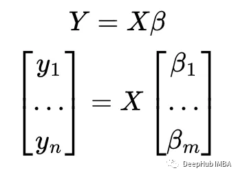
Y是一个长度为n的向量,由线性模型的目标值组成
β是一个长度为m的向量:这是模型必须“学习”的未知数。
X是形状为n行m列的数据矩阵。我们经常说我们有n个向量记录在m特征空间中
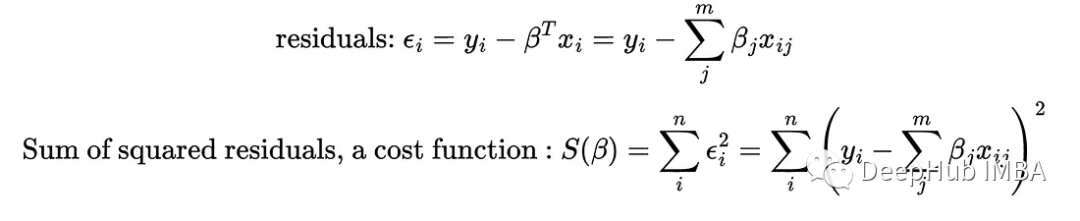
我们的目标是找到使平方误差最小的值
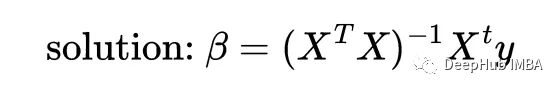
这个问题实际上有一个封闭形式的解,被称为普通最小二乘问题。解决方案是:
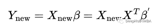
一旦解已知,就可以使用拟合模型计算新的y值给定新的x值,使用:
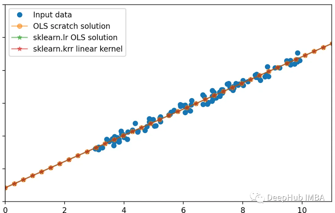
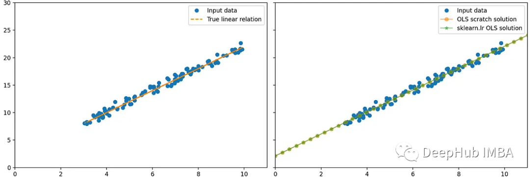
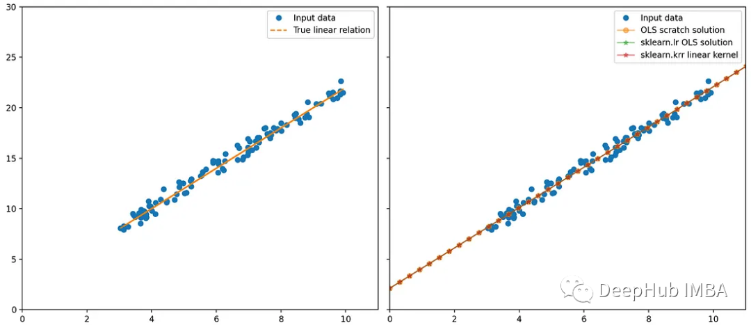
让我们用scikit-learn来验证我上面的数学理论:使用sklearn线性回归器,以及基于numpy的回归
 %matplotlib qt
 import numpy as np
 import matplotlib.pyplot as plt
 from sklearn.linear_model import LinearRegression

 np.random.seed(0)
 n = 100
 X_ = np.random.uniform(3, 10, n).reshape(-1, 1)
 beta_0 = 2
 beta_1 = 2
 true_y = beta_1 * X_ + beta_0
 noise = np.random.randn(n, 1) * 0.5 # change the scale to reduce/increase noise
 y = true_y + noise

 fig, axes = plt.subplots(1, 2, squeeze=False, sharex=True, sharey=True, figsize=(18, 8))
 axes[0, 0].plot(X_, y, "o", label="Input data")
 axes[0, 0].plot(X_, true_y, '--', label='True linear relation')
 axes[0, 0].set_xlim(0, 11)
 axes[0, 0].set_ylim(0, 30)
 axes[0, 0].legend()

 # f_0 is a column of 1s
 # f_1 is the column of x1
 X = np.c_[np.ones((n, 1)), X_]

 beta_OLS_scratch = np.linalg.inv(X.T @ X) @ X.T @ y
 lr = LinearRegression(
     fit_intercept=False, # do not fit intercept independantly, since we added the 1 column for this purpose
 ).fit(X, y)

 new_X = np.linspace(0, 15, 50).reshape(-1, 1)
 new_X = np.c_[np.ones((50, 1)), new_X]
 new_y_OLS_scratch = new_X @ beta_OLS_scratch
 new_y_lr = lr.predict(new_X)
 axes[0, 1].plot(X_, y, 'o', label='Input data')
 axes[0, 1].plot(new_X[:, 1], new_y_OLS_scratch, '-o', alpha=0.5,  label=r"OLS scratch solution")
 axes[0, 1].plot(new_X[:, 1], new_y_lr, '-*', alpha=0.5, label=r"sklearn.lr OLS solution")
 axes[0, 1].legend()
 fig.tight_layout()
 print(beta_OLS_scratch)
 print(lr.coef_)
可以看到,2种方法的结果是相同的
 [[2.12458946]
  [1.99549536]]
 [[2.12458946 1.99549536]]
这两种方法给出了相同的结果
核技巧 Kernel-trick
现在让我们回顾一种称为内核技巧的常用技术。
我们最初的问题(可以是任何类似分类或回归的问题)存在于输入数据矩阵X的空间中,在m个特征空间中有n个向量的形状。有时在这个低维空间中,向量不能被分离或分类,所以我们想要将输入数据转换到高维空间。可以手工完成,创建新特性。但是随着特征数量的增长,数值计算也将增加。
核函数的技巧在于使用设计良好的变换函数——通常是T或——从一个长度为m的向量x创建一个长度为m的新向量x ',这样我们的新数据具有高维数,并且将计算负荷保持在最低限度。
为了达到这个目的,函数必须满足一些性质,使得新的高维特征空间中的点积可以写成对应输入向量的函数——核函数:

这意味着高维空间中的内积可以表示为输入向量的函数。也就是说我们可以在高维空间中只使用低维向量来计算内积。这就是核技巧:可以从高维空间的通用性中获益,而无需在那里进行任何计算。
唯一的条件是我们只需要在高维空间中做点积。
实际上有一些强大的数学定理描述了产生这样的变换和/或这样的核函数的条件。
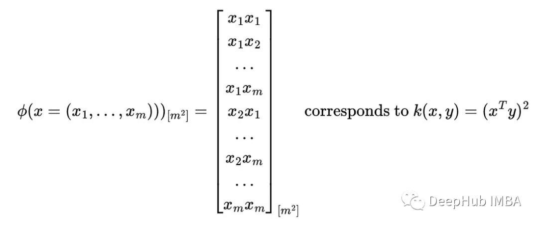
以下是一个核函数示例:
kernel从m维空间创建m^2维空间的第一个例子是使用以下代码:
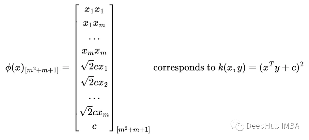
在核函数中添加一个常数会增加维数,其中包含缩放输入特征的新特征:
下面我们要用到的另一个核函数是线性核函数:
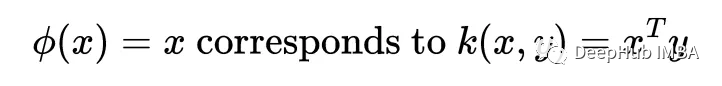
所以恒等变换等价于用一个核函数来计算原始空间的内积。
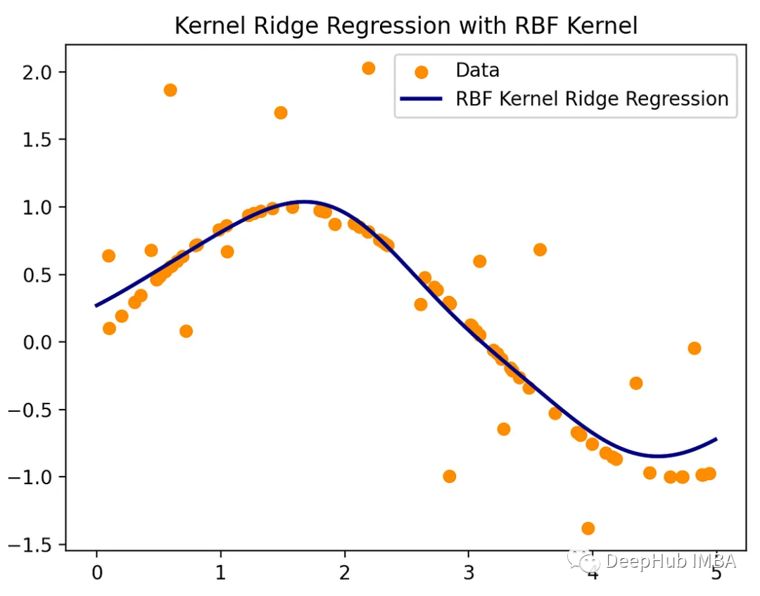
实际上还有很多其他有用的核,比如径向核(RBF)核或更一般的多项式核,它们可以创建高维和非线性特征空间。我们这里再简单介绍一个在线性回归环境中使用RBF核计算非线性回归的例子:
 import numpy as np
 from sklearn.kernel_ridge import KernelRidge
 import matplotlib.pyplot as plt

 np.random.seed(0)
 X = np.sort(5 * np.random.rand(80, 1), axis=0)
 y = np.sin(X).ravel()
 y[::5] += 3 * (0.5 - np.random.rand(16))

 # Create a test dataset
 X_test = np.arange(0, 5, 0.01)[:, np.newaxis]

 # Fit the KernelRidge model with an RBF kernel
 kr = KernelRidge(
     kernel='rbf', # use RBF kernel
     alpha=1, # regularization
     gamma=1, # scale for rbf
 )
 kr.fit(X, y)

 y_rbf = kr.predict(X_test)

 # Plot the results
 fig, ax = plt.subplots()
 ax.scatter(X, y, color='darkorange', label='Data')
 ax.plot(X_test, y_rbf, color='navy', lw=2, label='RBF Kernel Ridge Regression')
 ax.set_title('Kernel Ridge Regression with RBF Kernel')
 ax.legend()
线性回归中的线性核
如果变换将x变换为(x)那么我们可以写出一个新的线性回归问题
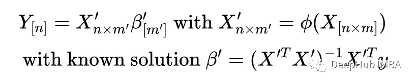
注意维度是如何变化的:线性回归问题的输入矩阵从[nxm]变为[nxm '],因此系数向量从长度m变为m '。
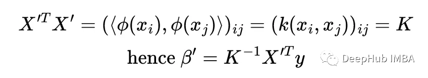
这就是核函数的诀窍:当计算解'时,注意到X '与其转置的乘积出现了,它实际上是所有点积的矩阵,它被称为核矩阵
线性核化和线性回归
最后,让我们看看这个陈述:在线性回归中使用线性核是无用的,因为它等同于标准线性回归。
线性核通常用于支持向量机的上下文中,但我想知道它在线性回归中的表现。
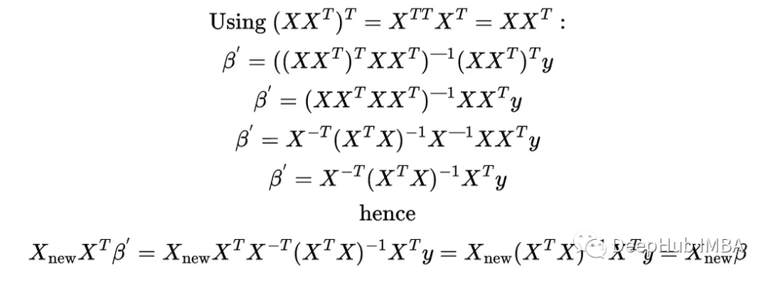
为了证明这两种方法是等价的,我们必须证明:
使用beta的第一种方法是原始线性回归,使用beta '的第二种方法是使用线性核化方法。我们可以用上面的矩阵性质和关系来证明这一点:
我们可以使用python和scikit learn再次验证这一点:
 %matplotlib qt
 import numpy as np
 import matplotlib.pyplot as plt
 from sklearn.linear_model import LinearRegression

 np.random.seed(0)
 n = 100
 X_ = np.random.uniform(3, 10, n).reshape(-1, 1)
 beta_0 = 2
 beta_1 = 2
 true_y = beta_1 * X_ + beta_0
 noise = np.random.randn(n, 1) * 0.5 # change the scale to reduce/increase noise
 y = true_y + noise

 fig, axes = plt.subplots(1, 2, squeeze=False, sharex=True, sharey=True, figsize=(18, 8))
 axes[0, 0].plot(X_, y, "o", label="Input data")
 axes[0, 0].plot(X_, true_y, '--', label='True linear relation')
 axes[0, 0].set_xlim(0, 11)
 axes[0, 0].set_ylim(0, 30)
 axes[0, 0].legend()

 # f_0 is a column of 1s
 # f_1 is the column of x1
 X = np.c_[np.ones((n, 1)), X_]

 beta_OLS_scratch = np.linalg.inv(X.T @ X) @ X.T @ y
 lr = LinearRegression(
     fit_intercept=False, # do not fit intercept independantly, since we added the 1 column for this purpose
 ).fit(X, y)

 new_X = np.linspace(0, 15, 50).reshape(-1, 1)
 new_X = np.c_[np.ones((50, 1)), new_X]
 new_y_OLS_scratch = new_X @ beta_OLS_scratch
 new_y_lr = lr.predict(new_X)
 axes[0, 1].plot(X_, y, 'o', label='Input data')
 axes[0, 1].plot(new_X[:, 1], new_y_OLS_scratch, '-o', alpha=0.5,  label=r"OLS scratch solution")
 axes[0, 1].plot(new_X[:, 1], new_y_lr, '-*', alpha=0.5, label=r"sklearn.lr OLS solution")
 axes[0, 1].legend()
 fig.tight_layout()
 print(beta_OLS_scratch)
 print(lr.coef_)
总结
在这篇文章中,我们回顾了简单线性回归,包括问题的矩阵公式及其解决方案。
然后我们介绍了了核技巧,以及它如何允许我们从高维空间中获益,并且不需要将低维数据实际移动到这个计算密集型空间。
最后,我证明了线性回归背景下的线性核实际上是无用的,它对应于简单的线性回归。
作者:Yoann Mocquin