关于Tacotron2看这一篇就够了

NATURAL TTS SYNTHESIS BY CONDITIONING WAVENET ON MEL SPECTROGRAM PREDICTIONS

文章来源

[1712.05884] NATURAL TTS SYNTHESIS BY CONDITIONING WAVENET ON MEL SPECTROGRAM PREDICTIONS

参考博客

声谱预测网络(Tacotron2)

Tacotron2 论文 + 代码详解

Tacotron2讲解

论文阅读 Tacotron2

Tacotron2 模型详解

Tacotron2-Details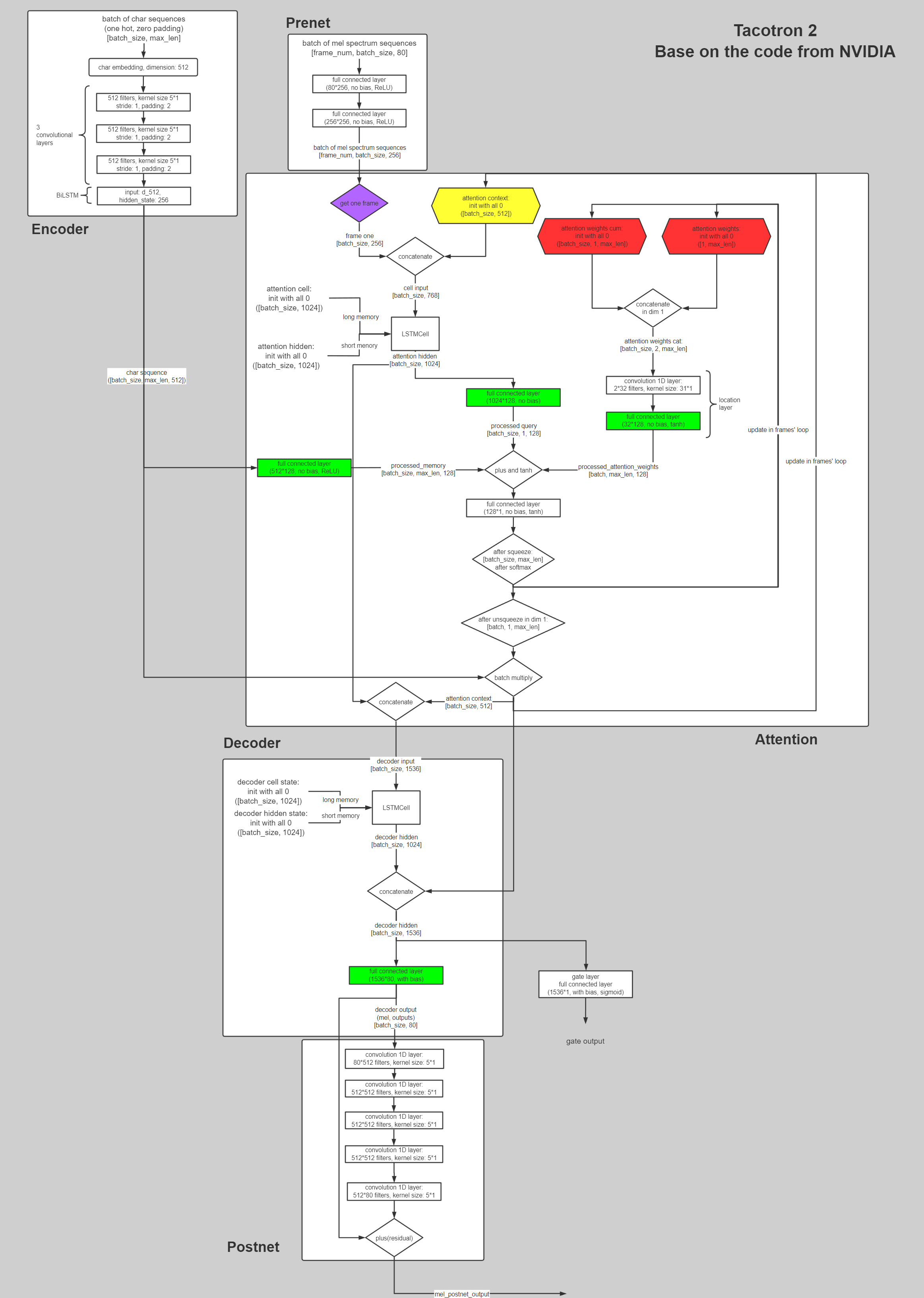

ABSTRUCT

简介：

The system is composed of a recurrent sequence-to-sequence feature prediction network that maps character embeddings to mel-scale spectrograms, followed by a modified WaveNet model acting as a vocoder to synthesize time-domain waveforms from those spectrograms.

模型由循环的seq2seq模型将character embeddings -> mel-scale spectrograms，之后使用一个改进的WaveNet模型作为vocoder生成时域波形。

MOS分数：

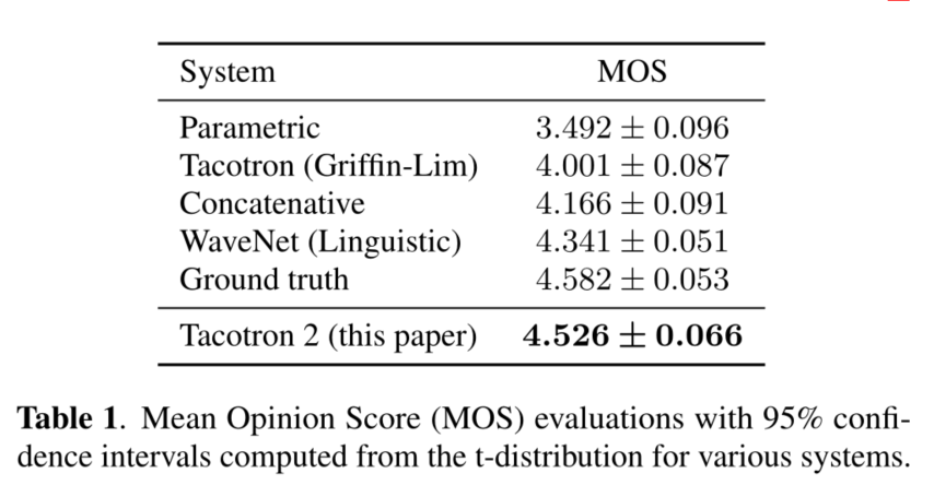
Our model achieves a mean opinion score (MOS) of 4.53 comparable to a MOS of 4.58 for professionally recorded speech.

消融分析：

To validate our design choices, we present ablation studies of key components of our system and evaluate the impact of using mel spectrograms as the conditioning input to WaveNet instead of linguistic, duration, and F0 features.

对使用mel图作为WaveNet的输入，而不是用linguistic、duration、F0 features的影响。

We further show that using this compact acoustic intermediate representation allows for a significant reduction in the size of the WaveNet architecture.

表明使用mel图作为中间表示可以减少WaveNet框架的尺寸。

1. INTRODUCTION

在TTS各个发展阶段存在的问题：

Over time, different techniques have dominated the field.

Concatenative synthesis with unit selection, the process of stitching small units of pre-recorded waveforms together [2, 3] was the state-of-the-art for many years.

Statistical parametric speech synthesis [4, 5, 6, 7], which directly generates smooth trajectories of speech features to be synthesized by a vocoder, followed, solving many of the issues that concatenative synthesis had with boundary artifacts.

However, the audio produced by these systems often sounds muffled and unnatural compared to human speech.

在不同时期，不同的TTS技术占据主导地位，但是无论是Concatenative Synthesis还是SPSS都存在一个问题，就是这些系统产生的音频和人类语音相比，往往听起来很沉闷、不自然。

WaveNet介绍：

WaveNet [8], a generative model of time domain waveforms, produces audio quality that begins to rival that of real human speech and is already used in some complete TTS systems [9, 10, 11].

WaveNet，产生时域波形的模型，产生的音频质量可以和真是人类的语音相媲美，并且已经应用在一些完整的TTS系统中。

WaveNet的一些问题：

The inputs to WaveNet (linguistic features, predicted log fundamental frequency (F0), and phoneme durations), however, require significant domain expertise to produce, involving elaborate text-analysis systems as well as a robust lexicon (pronunciation guide).

WaveNet输入的是像linguistic features, predicted log fundamental frequency (F0), and phoneme durations，这些输入需要大量的领域专业知识才能使用，这些专业知识包括精心设计的文本分析系统和robust词汇表(发音指南)。

Tacotron介绍：

Tacotron [12], a sequence-to-sequence architecture [13] for producing magnitude spectrograms from a sequence of characters, simplifies the traditional speech synthesis pipeline by replacing the production of these linguistic and acoustic features with a single neural network trained from data alone.

To vocode the resulting magnitude spectrograms, Tacotron uses the Griffin-Lim algorithm [14] for phase estimation, followed by an inverse short-time Fourier transform.

Tacotron，是一个序列到序列的结构，可以从一系列的字符产生频谱图，简化了传统语音合成流程，仅仅根据数据训练的单个网络来代替了语言和声学特征。Tacotron使用Griffin-Lim算法进行相位估计，然后在进行反短时傅里叶变换将mel图转为wavefrom。与WaveNet等方法相比，Griffin-Lim会产生特有的伪影和较低的音频质量。

Tacotron2介绍：

In this paper, we describe a unified, entirely neural approach to speech synthesis that combines the best of the previous approaches: a sequence-to-sequence Tacotron-style model [12] that generates mel spectrograms, followed by a modified WaveNet vocoder [10, 15].

Tacotron2仍然使用了一个seq2seq的Tacotron模型，通过这个模型产生mel图，将mel图输入改进的WaveNet Vocoder生成波形。

优点：

Trained directly on normalized character sequences and corresponding speech waveforms, our model learns to synthesize natural sounding speech that is difficult to distinguish from real human speech.

直接对规范化的<text, audio>对进行训练，Tacotron可以合成非常自然的语音(几乎很难和真实的人类语音相区别)。

2. MODEL ARCHITECTURE

Tacotron2的主要组成部分：

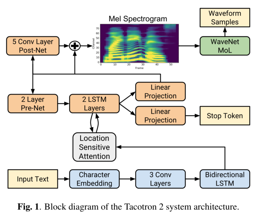
Our proposed system consists of two components, shown in Figure 1:

1. A recurrent sequence-to-sequence feature prediction network with attention which predicts a sequence of mel spectrogram frames from an input character sequence.
2. A modified version of WaveNet which generates time-domain waveform samples conditioned on the predicted mel spectrogram frames.

2.1 Intermediate Feature Representation

Tacotron2模型中的中间特征表示：

In this work we choose a low-level acoustic representation: mel-frequency spectrograms, to bridge the two components.

mel-frequency spectrograms介绍

A mel-frequency spectrogram is related to the linear-frequency spectrogram, i.e., the short-time Fourier transform (STFT) magnitude.

梅尔频谱图和线性频谱图相关，即STFT的幅度。

It is obtained by applying a nonlinear transform to the frequency axis of the STFT, inspired by measured responses from the human auditory system, and summarizes the frequency content with fewer dimensions.

梅尔频谱图是通过对STFT的频率轴做非线性变换得到的。

使用mel-frequency spectrograms的优势：

Using a representation that is easily computed from time-domain waveforms allows us to train the two components separately.

使用时域波形计算的表示形式，我们可以更加容易地分别训练两个组件。

This representation is also smoother than waveform samples and is easier to train using a squared error loss because it is invariant to phase within each frame.

mel频谱图表示也比波形样本更加平滑，而且使用平方误差损失也更好训练，因为它在每一帧内的相位都是不变的。

Griffin-Lim使用线性频谱图生成波形图：

While linear spectrograms discard phase information (and are therefore lossy), algorithms such as Griffin-Lim are capable of estimating this discarded information, which enables time-domain conversion via the inverse short-time Fourier transform.

虽然线性谱图丢弃了相位信息（因此是有损失的），但Griffin-Lim等算法能够估计这些被丢弃的信息，从而通过反短时傅里叶变换实现时域转换。

改进的WaveNet将mel频谱图生成波形图：

Mel spectrograms discard even more information, presenting a challenging inverse problem.

梅尔频谱图丢弃的信息更多，提出了一个具有挑战性的逆向问题。

However, in comparison to the linguistic and acoustic features used in WaveNet, the mel spectrogram is a simpler, lowerlevel acoustic representation of audio signals.

然而，与WaveNet中使用的语言和声学特征相比，梅尔频谱图是一种更简单、更低级的音频信号声学表示。

It should therefore be straightforward for a similar WaveNet model conditioned on mel spectrograms to generate audio, essentially as a neural vocoder.

因此，类似的WaveNet模型以梅尔频谱图为输入，基本上是作为一个神经声码器来生成音频。

Indeed, we will show that it is possible to generate high quality audio from mel spectrograms using a modified WaveNet architecture.

使用修改后的WaveNet结构，有可能从梅尔频谱图中生成高质量的音频。

2.2. Spectrogram Prediction Network

生成mel频谱图：

As in Tacotron, mel spectrograms are computed through a short-time Fourier transform (STFT) using a 50 ms frame size, 12.5 ms frame hop, and a Hann window function.

与Tacotron一样，mel频谱图是通过短时傅里叶变换（STFT）计算的，使用50毫秒的帧大小，12.5毫秒的帧跳，以及一个Hann窗口函数。

We experimented with a 5 ms frame hop to match the frequency of the conditioning inputs in the original WaveNet, but the corresponding increase in temporal resolution resulted in significantly more pronunciation issues.

当使用5毫秒的帧跳来匹配原始WaveNet中调节输入的频率，但时间分辨率的相应增加导致了明显更多的发音问题。

We transform the STFT magnitude to the mel scale using an 80 channel mel filterbank spanning 125 Hz to 7.6 kHz, followed by log dynamic range compression.

使用一个横跨125Hz到7.6kHz的80通道梅尔滤波器库将STFT幅度转换为梅尔尺度，然后进行对数动态范围压缩。

Prior to log compression, the filterbank output magnitudes are clipped to a minimum value of 0.01 in order to limit dynamic range in the logarithmic domain.

在对数压缩之前，滤波器库的输出幅度被压缩到最小值0.01，以限制对数域的动态范围。

mel频谱图预测网络的构成：

The network is composed of an encoder and a decoder with attention.

频谱预测网络主要由一个编码器和一个带有注意力的解码器组成。

The encoder converts a character sequence into a hidden feature representation which the decoder consumes to predict a spectrogram.

编码器将字符序列转换为隐藏的特征表示，解码器使用这些特征来预测谱图。

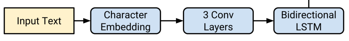
1. Encoder

Input characters are represented using a learned 512-dimensional character embedding, which are passed through a stack of 3 convolutional layers each containing 512 filters with shape 5 × 1, i.e., where each filter spans 5 characters, followed by batch normalization [18] and ReLU activations.

1. 输入的数据维度为[batch_size, char_seq_length]
2. 使用512维的Character Embedding，把每个character映射为512维的向量，输出维度为[batch_size, char_seq_length, 512]
3. 3个一维卷积，每个卷积包括512个kernel，每个kernel的大小是5x1（即每次看5个characters）。每做完一次卷积，进行一次BatchNorm、ReLU以及Dropout。输出维度为[batch_size, char_seq_length, 512]（为了保证每次卷积的维度不变，因此使用了padding），这里使用卷积层获取上下文主要是由于实践中RNN很难捕获长时依赖。F1、F2、F3为3个卷积核，ReLU为每一个卷积层上的非线性激活，E表示对字符序列X做embedding

As in Tacotron, these convolutional layers model longer-term context (e.g., N-grams) in the input character sequence.

像在Tacotron中一样，这些卷积层(使用像n-grams)在输入字符序列中模拟长句子上下文。

The output of the final convolutional layer is passed into a single bi-directional [19] LSTM [20] layer containing 512 units (256 in each direction) to generate the encoded features.

1. 上面得到的输出，扔给一个单层BiLSTM（用于生成编码特征），隐藏层维度是256，由于这是双向的LSTM，因此最终输出维度是[batch_size, char_seq_length, 512]

2. Location sensitive attention

The encoder output is consumed by an attention network which summarizes the full encoded sequence as a fixed-length context vector for each decoder output step.

Encoder的输出作为Attention的输入，Attention将完整的Encoder序列总结为每个decoder输出step上的固定长度的上下文向量。

We use the location-sensitive attention from [21], which extends the additive attention mechanism [22] to use cumulative attention weights from previous decoder time steps as an additional feature.

我们使用位置敏感注意力，它扩展了加法注意力机制，将以前Decoder时间步的累积注意力权重作为一个额外的特征。

This encourages the model to move forward consistently through the input, mitigating potential failure modes where some subsequences are repeated or ignored by the decoder.

这鼓励了模型通过输入持续前进，减轻了一些子序列被重复或被解码器忽略的潜在失败形式。

Attention probabilities are computed after projecting inputs and location features to 128-dimensional hidden representations.

注意力概率是在将输入和位置特征投射到128维的隐藏表征后计算出来的。

Location features are computed using 32 1-D convolution filters of length 31.

位置特征是用32个长度为31的一维卷积filter计算的。

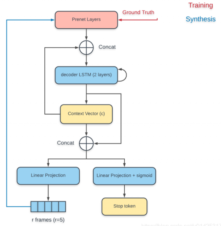
3. Decoder

The decoder is an autoregressive recurrent neural network which predicts a mel spectrogram from the encoded input sequence one frame at a time.

解码器是一个自回归循环神经网络，它从编码的输入序列预测输出声谱图，一次预测一帧。

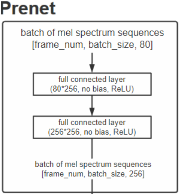
1. pre-netThe prediction from the previous time step is first passed through a small pre-net containing 2 fully connected layers of 256 hidden ReLU units.We found that the pre-net acting as an information bottleneck was essential for learning attention.上一个时间步预测出的频谱首先传入到一个pre-net，其中包含2个完全连接的256个隐藏的ReLU单元层，PreNet作为一个信息瓶颈层（bottleneck），对于学习注意力是必要的。
2. LSTMThe prenet output and attention context vector are concatenated and passed through a stack of 2 unidirectional LSTM layers with 1024 units.PreNet的输出和Attention Context向量拼接在一起，传给一个含有1024个单元的两层单向LSTM。
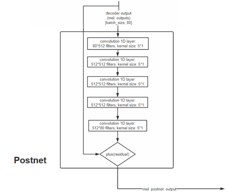
3. post-net + Linear ProjectionThe concatenation of the LSTM output and the attention context vector is projected through a linear transform to predict the target spectrogram frame.LSTM的输出再次和Attention Context向量拼接在一起，然后经过一个线性投影来预测目标频谱。Finally, the predicted mel spectrogram is passed through a 5-layer convolutional post-net which predicts a residual to add to the prediction to improve the overall reconstruction.最后，目标频谱帧经过一个5层卷积的post-net（后处理网络），再将该输出和Linear Projection的输出相加（残差连接）作为最终的输出。Each post-net layer is comprised of 512 filters with shape 5 × 1 with batch normalization, followed by tanh activations on all but the final layer.每一层post-net都由512个5x1的filter组成，在输出时进行BN，并在除最后一层以外的所有层上使用tanh作为激活函数。We minimize the summed mean squared error (MSE) from before and after the post-net to aid convergence我们将后处理网络前后的平均平方误差（MSE）之和降到最低，以帮助收敛。
4. Linear Projection + sigmoidIn parallel to spectrogram frame prediction, the concatenation of decoder LSTM output and the attention context is projected down to a scalar and passed through a sigmoid activation to predict the probability that the output sequence has completed.另一边，LSTM的输出和Attention Context向量拼接在一起，投影成标量后传给sigmoid激活函数，来预测输出序列是否已完成预测的概率。This “stop token” prediction is used during inference to allow the model to dynamically determine when to terminate generation instead of always generating for a fixed duration.这种 "停止标记 "的预测在推理过程中被使用，使模型能够动态地确定何时终止生成，而不是总是给定一个固定的停止时间。Specifically, generation completes at the first frame for which this probability exceeds a threshold of 0.5.具体来说，在这个概率超过0.5的阈值的第一帧就完成了生成。
5. DetailThe convolutional layers in the network are regularized using dropout [25] with probability 0.5, and LSTM layers are regularized using zoneout [26] with probability 0.1.网络中的卷积层使用概率为0.5的dropout[25]进行规范化，LSTM层使用概率为0.1的zoneout[26]进行规范化。In order to introduce output variation at inference time, dropout with probability 0.5 is applied only to layers in the pre-net of the autoregressive decoder.为了在推理时引入输出变化，概率为0.5的dropout只适用于自回归解码器的预处理网络中的层。

Tacotron1和Tacotron2的重点区别：

1. encoder部分，使用了embedding + 3Conv_layers + Bi-directional_LSTM
2. attention使用的是location sensitive attention
3. Pre_net的dropout是一直设置为 true 的（据说是根据实验效果），post_net中最后一层一般为linear激活函数
4. 最后的 mel_output_post 是经过 post_net 和 linear_projection相加得到
5. 多帧预测方面，虽然Tacotron2没有使用多帧，但是实现原理类似

2.3. WaveNet Vocoder

改进的WaveNet架构：

We use a modified version of the WaveNet architecture from [8] to invert the mel spectrogram feature representation into time-domain waveform samples.

使用改进的WaveNet，将mel图转为表示时域的波形样本。

扩张卷积(dilated convolution)

As in the original architecture, there are 30 dilated convolution layers, grouped into 3 dilation cycles, i.e., the dilation rate of layer k (k = 0 . . . 29) is

与原始WaveNet结构一样，有30个扩张卷积层，分为3个扩张周期，即第k层(k=0 … 29)的扩张率为。

To work with the 12.5 ms frame hop of the spectrogram frames, only 2 upsampling layers are used in the conditioning stack instead of 3 layers.

为了配合频谱图帧的12.5毫秒帧跳，在调节堆叠中只使用2个上采样层，而不是3个层。

Instead of predicting discretized buckets with a softmax layer, we follow PixelCNN++ [27] and Parallel WaveNet [28] and use a 10 component mixture of logistic distributions (MoL) to generate 16-bit samples at 24 kHz.

*没有使用softmax层预测离散片段，而是借鉴了PixelCNN++[27]和Parallel WaveNet[28]，使用10元混合逻辑分布(10-component MoL)来产生24kHz的16位深的语音样本。*

To compute the logistic mixture distribution, the WaveNet stack output is passed through a ReLU activation followed by a linear projection to predict parameters (mean, log scale, mixture weight) for each mixture component.

为了计算混合逻辑分布，WaveNet的堆叠输出传给ReLU激活函数，再连接一个线性投影层来预测每一个混元预测参数（均值，对数刻度，混合权重）。

The loss is computed as the negative log-likelihood of the ground truth sample.

损失函数使用标定真实数据的负对数似然函数计算而得。

3. EXPERIMENTS & RESULTS

3.1. Training Setup

训练过程

Our training process involves first training the feature prediction network on its own, followed by training a modified WaveNet independently on the outputs generated by the first network.

先单独训练特征预测网络，之后使用特征预测网络产生的输出独立训练一个修改过的WaveNet。

1. 训练特征预测网络(Encoder+Attention+Decoder)

To train the feature prediction network, we apply the standard maximum-likelihood training procedure (feeding in the correct output instead of the predicted output on the decoder side, also referred to as teacher-forcing) with a batch size of 64 on a single GPU.

为了训练特征预测网络，我们在单个GPU上指定batch size为64，使用标准的最大似然训练步骤（在解码器端不是传入预测结果而是传入正确的结果，这种方法也被称为teacher-forcing）。

We use the Adam optimizer [29] with β1 = 0.9, β2 = 0.999, ε = 10^−6 and a learning rate of 10^−3 exponentially decaying to 10^−5 starting after 50,000 iterations.

我们使用Adam优化器[29]，β1 = 0.9, β2 = 0.999, ε = 10-6，学习率为10-3，在50,000次迭代后开始指数式衰减到10-5。

We also apply L2 regularization with weight 10^−6.

我们还应用权重为10^-6的L2正则化。

2. 训练修改后的WaveNet

We then train our modified WaveNet on the ground truth-aligned predictions of the feature prediction network.

之后，我们把特征预测网络输出的预测结果与标定数据对齐，使用经过对齐处理的预测结果来训练改良版的WaveNet。

That is, the prediction network is run in teacher-forcing mode, where each predicted frame is conditioned on the encoded input sequence and the corresponding previous frame in the ground truth spectrogram.

This ensures that each predicted frame exactly aligns with the target waveform samples.

也就是说这些预测数据是在teacher-forcing模式下产生的：所预测的每一帧是基于编码的输入序列以及所对应的前一帧标定数据频谱。这保证了每个预测帧与目标波形样本完全对齐。

We train with a batch size of 128 distributed across 32 GPUs with synchronous updates, using the Adam optimizer with β1 = 0.9, β2 = 0.999, ? = 10−8 and a fixed learning rate of 10−4.

在训练过程中，使用Adam优化器并指定参数β1 = 0.9; β2 = 0.999; ε= 1e-8，学习率固定为10e-4，把batch size为128的批训练分布在32个GPU上执行并同步更新。

It helps quality to average model weights over recent updates.

这有助于使用最近的更新来优化平均模型权重。

Therefore we maintain an exponentially-weighted moving average of the network parameters over update steps with a decay of 0.9999 – this version is used for inference (see also [29]).

所以我们在更新网络参数时采用衰减率为0.9999的指数加权平均 – 这个处理用在推断中（请参照[29]）。

To speed up convergence, we scale the waveform targets by a factor of 127.5 which brings the initial outputs of the mixture of logistics layer closer to the eventual distributions.

为了加速收敛，我们用127.5的缩放因子来放大目标波形，这使得混合逻辑层的初始输出更接近最终分布。

3. 训练使用的数据集

We train all models on an internal US English dataset[12], which contains 24.6 hours of speech from a single professional female speaker.

我们在一个内部的美国英语数据集上训练所有的模型，该数据集包含了一个专业女性演讲者24.6小时的语音。

All text in our datasets is spelled out. e.g., “16” is written as “sixteen”, i.e., our models are all trained on normalized text.

并且数据集中的所有文本都进行了文本规范化。

3.2. Evaluation

When generating speech in inference mode, the ground truth targets are not known.

Therefore, the predicted outputs from the previous step are fed in during decoding, in contrast to the teacher-forcing configuration used for training.

在推理阶段生成语音的时候，是没有标定数据的，所以与训练的时候不一样，就直接在解码处理中传入上一步的预测结果。

对比实验：

1. 评估集

We randomly selected 100 fixed examples from the test set of our internal dataset as the evaluation set.

Note that while instances in the evaluation set never appear in the training set, there are some recurring patterns and common words between the two sets.

请注意，虽然评估集中的实例从未出现在训练集中，但在这两个集合之间有一些重复出现的模式和共同的词语。

Since all the systems we compare are trained on the same data, relative comparisons are still meaningful.

由于我们比较的所有系统都是在相同的数据上训练出来的，所以相对比较仍然是有意义的。

2. MOS分数

Audio generated on this set are sent to a human rating service similar to Amazon’s Mechanical Turk where each sample is rated by at least 8 raters on a scale from 1 to 5 with 0.5 point increments, from which a subjective mean opinion score (MOS) is calculated.

在这个集合上产生的音频被送到一个类似于亚马逊的Mechanical Turk的人类评分服务系统中，每个样本由至少8个评分者在1到5分的范围内进行评分(以0.5分的增量)，从中计算出一个主观的平均意见分数（MOS）。

Each evaluation is conducted independently from each other, so the outputs of two different models are not directly compared when raters assign a score to them.

每个评价都是独立进行的，所以当评分者给两个不同的模型打分时，两个模型的输出并不直接比较。

Tacotron2与之间各种生成方法的比较：

1. MOS分数对比

为了去除由于mel图造成的误差，加入了Tacotron2和原始WaveNet的比对。

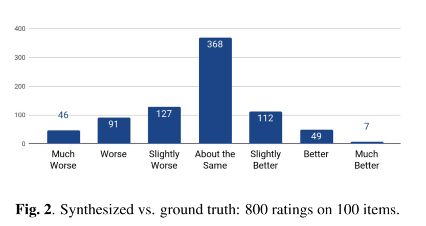
2. 将系统合成的音频和ground truth进行并排评估

For each pair of utterances, raters are asked to give a score ranging from -3 (synthesized much worse than ground truth) to 3 (synthesized much better than ground truth).

对于每一对<synthesized, ground truth>进行评分，评分范围[-3, 3]。-3分表示合成的语音比真实的相差很多，3分表示合成的语音比真实语音更优秀。

结果

The overall mean score of −0.270 ± 0.155 shows that raters have a small but statistically significant preference towards ground truth over our results.

The comments from raters indicate that occasional mispronunciation by our system is the primary reason for this preference.

结果为−0.270 ± 0.155，说明真实的语音要强于合成的语音。

造成该结果的原因：合成语音中由偶尔的错误发音。

3. 在附件E中的测试集中评估MOS值

We ran a separate rating experiment on the custom 100-sentence test set from Appendix E of [11], obtaining a MOS of 4.354.

These results show that while our system is able to reliably attend to the entire input, there is still room for improvement in prosody modeling.

这些结果表明，该系统能够可靠地注意到整个输入，但韵律建模方面仍有改进的空间。

4. 测试系统对域外文本的概括能力

Finally, we evaluate samples generated from 37 news headlines to test the generalization ability of our system to out-of-domain text.

我们评估了从37个新闻头条中产生的样本，以测试我们的系统对域外文本的概括能力。

On this task, our model receives a MOS of 4.148±0.124 while WaveNet conditioned on linguistic features receives a MOS of 4.137 ± 0.128.

在这项任务中，我们的模型获得了4.148±0.124的MOS，而以语言特征为条件的WaveNet获得了4.137±0.128的MOS。

结论

Examination of rater comments shows that our neural system tends to generate speech that feels more natural and human-like, but it sometimes runs into pronunciation difficulties, e.g., when handling names.

该神经系统倾向于产生感觉更自然、更像人类的语音，但它有时会遇到发音困难，例如在处理名字时。

This result points to a challenge for end-to-end approaches – they require training on data that cover intended usage.

这个结果指出了端到端方法的一个挑战–它们需要在涵盖预期用途的数据上进行训练。

3.3. Ablation Studies

3.3.1. Predicted Features versus Ground Truth

Tacotron2模型中的两个部分是分开训练的，但是对改进的WaveNet进行训练需要Spectrogram Prediction Network中预测的特征。

在消融研究中，我们使用了从ground truth中提取的mel图对WaveNet进行训练。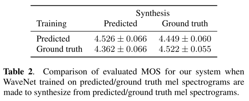

结果：

1. 当训练和推理使用的特征相同时，会得到最好的性能。
2. 当使用ground truth进行训练，并且使用预测的特征进行合成时，得到的结果反而更差。原因：预测的频谱图过度平滑，没有ground truth详细。当使用ground truth进行训练时，网络没有学会如何从过度平滑的特征中生成高质量的语音波形。

3.3.2. Linear Spectrograms

在实验中尝试使用线性频谱图来代替mel频谱图，从而使用Griffin-Lim生成波形。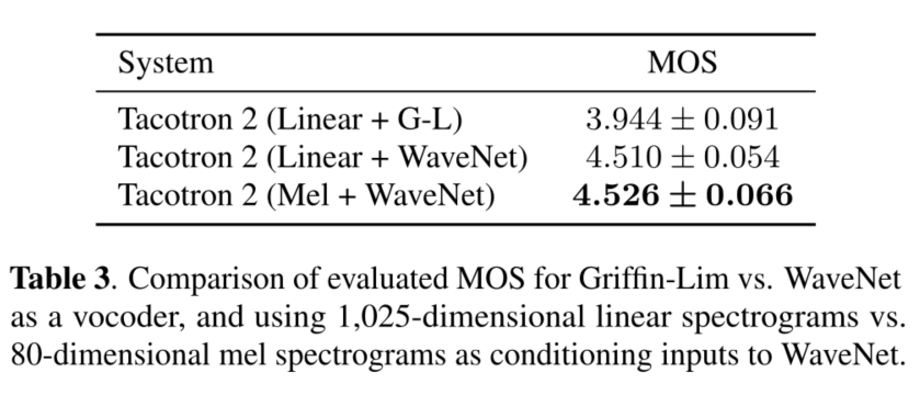

3.3.3. Post-Processing Network

Since it is not possible to use the information of predicted future frames before they have been decoded, we use a convolutional post-processing network to incorporate past and future frames after decoding to improve the feature predictions.

由于在未来帧被解码之前不可能被当作信息使用，所以使用post-net，在解码后纳入过去和未来的帧，以改善特征预测。

在改进的WaveNet中包含了卷积层，所以在使用改进的WaveNet作为Vocoder时post-net是否还有必要？

To answer this question, we compared our model with and without the post-net, and found that without it, our model only obtains a MOS score of 4.429 ± 0.071, compared to 4.526 ± 0.066 with it, meaning that empirically the post-net is still an important part of the network design.

为了回答这个问题，我们比较了有无后置网络的模型，发现如果没有后置网络，我们的模型只获得了4.429±0.071的MOS分数，而有了后置网络则获得了4.526±0.066的分数，这意味着根据经验，后置网络仍然是网络设计的一个重要部分。

3.3.4. Simplifying WaveNet

WaveNet中的一个决定性特征是其使用了dilated convolution。

在实验中评估了具有不同感受野大小和层数的模型，以测试我们的假设，即具有小感受野的浅层网络可能也会有一个令人满意的结果。原因是mel图比语言特征更接近波形，并且捕获了跨帧的长期依赖关系。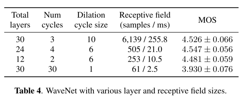

表4表明，大的感受野不是决定音频质量的基本因素。

但在另一方面，如果我们完全不使用扩张卷积，即使堆栈的深度和baseline相同，但是感受野就会比baseline小两个数量级，并且质量也会明显下降。

4. CONCLUSION

This paper describes Tacotron 2, a fully neural TTS system that combines a sequence-to-sequence recurrent network with attention to predicts mel spectrograms with a modified WaveNet vocoder.

本文介绍了Tacotron 2，一个完全的神经TTS系统，它将一个序列到序列的递归网络与注意预测熔体谱图与一个修改的WaveNet声码相结合。

The resulting system synthesizes speech with Tacotron-level prosody and WaveNet-level audio quality.

该系统合成的语音和Tacotron具有相同的韵律水平、和WaveNet具有相同水平的音频质量。

This system can be trained directly from data without relying on complex feature engineering, and achieves state-of-the-art sound quality close to that of natural human speech.

这个系统可以直接从数据中进行训练，而不需要依赖复杂的特征工程，并实现了接近人类自然语音的最先进的声音质量。