
1 Ornstein-Uhlenbeck过程
用SDE的形式表示,Ornstein-Uhlenbeck过程为:
- θ就是均值回归的速率(θ越大,干扰越小)
- μ是均值
- σ是波动率(扰动的程度)
- ε ~N(0,1)
从SDE的角度看,随机过程包含两块:
- 第一部分表示均值回归,即不论如何变化,下一时刻总会朝着均值方向变化
- 第二部分就是一个布朗运动生成的随机项
1.1 解析解推导
定义
,根据伊藤引理,有:
数学知识整理:布朗运动与伊藤引理 (Ito‘s lemma)_UQI-LIUWJ的博客-CSDN博客
![=(\theta X_t e^{\theta t}+[\theta(\mu-X_t)]e^{\theta t}+\frac{1}{2}\sigma^2 \cdot 0)dt+e^{\theta t} \sigma \epsilon \sqrt{dt}](https://latex.codecogs.com/gif.latex?%3D%28%5Ctheta%20X_t%20e%5E%7B%5Ctheta%20t%7D+%5B%5Ctheta%28%5Cmu-X_t%29%5De%5E%7B%5Ctheta%20t%7D+%5Cfrac%7B1%7D%7B2%7D%5Csigma%5E2%20%5Ccdot%200%29dt+e%5E%7B%5Ctheta%20t%7D%20%5Csigma%20%5Cepsilon%20%5Csqrt%7Bdt%7D) 
然后我们计算
 将
移到等号右边去,同时等号左右同时除以
(
的系数)
有:
又根据伊藤等距,有:数学知识整理:布朗运动与伊藤引理 (Ito‘s lemma)_UQI-LIUWJ的博客-CSDN博客
然后因为
,所以
1.2 离散解
如果我们考虑离散形式,记单步step为τ:

形式上就是 ,也即自回归形式AR(1)
1.2.1 离散解在RL中的延申
    通过上一小段,不难发现Ornstein-Uhlenbeck过程是时序相关的【且满足马尔科夫性,后一步的噪声仅受前一步的影响】,所以在强化学习的前一步和后一步的动作选取过程中可以**利用Ornstein-Uhlenbeck过程产生时序相关的噪声**,以提高在惯性系统(环境)中的控制任务的探索效率。【上一步的噪声和下一步的噪声之间是有单步自回归的关系)

    常用的高斯噪声是时序上不相关的,前一步和后一步选取动作的时候噪声都是独立的。

    ——>相比于独立噪声,**OU噪声适合于惯性系统,尤其是时间离散化粒度较小的情况 **(时间离散化粒度大的时候,可能OU噪声和高斯噪声的区别就不明显了)

            ——>在惯性系统中,如果使用高斯噪声,那么会产生一系列独立的在0均值附近的高斯噪声,原地震荡,使得随机噪声的作用被平均/抵消了

            ——>如果使用OU噪声的话,会顺着惯性往一个方向多探索几步,这样可以累计探索的效果
2 代码实现
import numpy as np
import matplotlib.pyplot as plt

class Ornstein_Uhlenbeck_Noise:
    def __init__(self, mu, sigma=1.0, theta=0.15, dt=1e-2, x0=None):
        self.theta = theta
        self.mu = mu
        self.sigma = sigma
        self.dt = dt
        self.x0 = x0
        self.reset()

    def __call__(self):
        x = self.x_prev + \
            self.theta * (self.mu - self.x_prev) * self.dt + \
            self.sigma * np.sqrt(self.dt) * np.random.normal(size=self.mu.shape)
        '''
        后两行是dXt,其中后两行的前一行是θ(μ-Xt)dt,后一行是σεsqrt(dt)
        '''
        self.x_prev = x
        return x

    def reset(self):
        if self.x0 is not None:
            self.x_prev = self.x0
        else:
            self.x_prev = np.zeros_like(self.mu)
2.1 和高斯噪声的比较
ou_noise = Ornstein_Uhlenbeck_Noise(mu=np.zeros(1))
y1 = []
y2 = np.random.normal(0, 1, 1000) #高斯噪声
for _ in range(1000):
        y1.append(ou_noise())
fig,ax=plt.subplots(1,2,figsize=(10,5))
ax[0].plot(y1, c='r')
ax[0].set_title('OU noise')
ax[1].plot(y2, c='b')
ax[1].set_title('Guassian noise')
plt.show()

可以看到OU噪声是一个有一定自回归的噪声,而高斯噪声是两两独立的
OU noise往往不会高斯噪声一样相邻的两步的值差别那么大,而是会绕着均值依据惯性在上一步附近正向或负向探索一段距离,就像物价和利率的波动一样,这有利于在一个方向上探索。
2.2 不同参数的影响
2.2.1 sigma
if __name__ == "__main__":
    ou_noise1 = Ornstein_Uhlenbeck_Noise(sigma=1,mu=np.zeros(1))
    ou_noise2 = Ornstein_Uhlenbeck_Noise(sigma=0.1,mu=np.zeros(1))
    y1 = []
    y2 = []
    for _ in range(1000):
        y1.append(ou_noise1())
        y2.append(ou_noise2())
    fig,ax=plt.subplots(1,2,figsize=(10,5))
    ax[0].plot(y1, c='r')
    ax[0].set_title('OU noise_sigma=1')
    ax[1].plot(y2, c='b')
    ax[1].set_title('OU noise_sigma=0.1')
    plt.show()
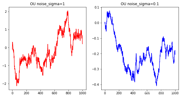
σ大,那么扰动就会大一些
2.2.2 dt
if __name__ == "__main__":
    ou_noise1 = Ornstein_Uhlenbeck_Noise(dt=1e-2,mu=np.zeros(1))
    ou_noise2 = Ornstein_Uhlenbeck_Noise(dt=1,mu=np.zeros(1))
    y1 = []
    y2 = []
    for _ in range(1000):
        y1.append(ou_noise1())
        y2.append(ou_noise2())
    fig,ax=plt.subplots(1,2,figsize=(10,5))
    ax[0].plot(y1, c='r')
    ax[0].set_title('OU noise_dt=1e-2')
    ax[1].plot(y2, c='b')
    ax[1].set_title('OU noise_dt=1')
    plt.show()
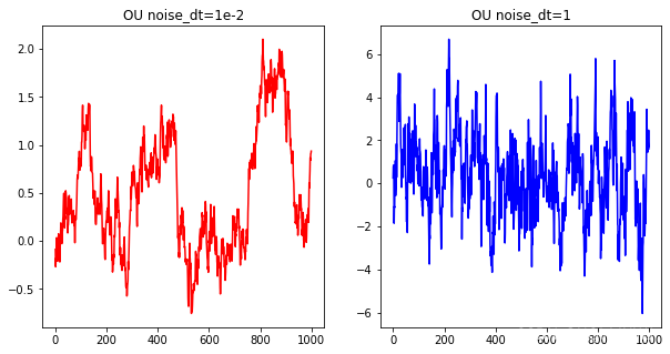
这也印证了前面1.2.1的说法:时间离散化粒度大的时候,可能OU噪声和高斯噪声的区别就不明显了【这可能是很多地方说OU噪声没有作用的一个原因。。。】
2.2.3 theta
if __name__ == "__main__":
    ou_noise1 = Ornstein_Uhlenbeck_Noise(theta=0.15,mu=np.zeros(1))
    ou_noise2 = Ornstein_Uhlenbeck_Noise(theta=1,mu=np.zeros(1))
    y1 = []
    y2 = []
    for _ in range(1000):
        y1.append(ou_noise1())
        y2.append(ou_noise2())
    fig,ax=plt.subplots(1,2,figsize=(10,5))
    ax[0].plot(y1, c='r')
    ax[0].set_title('OU noise_theta=0.15')
    ax[1].plot(y2, c='b')
    ax[1].set_title('OU noise_theta=1')
    plt.show()

θ大,那么向均值考虑的程度就会更猛烈一些
参考内容
强化学习中Ornstein-Uhlenbeck噪声是鸡肋吗? - 知乎 (zhihu.com)
本文转载自: https://blog.csdn.net/qq_40206371/article/details/125713187
版权归原作者 UQI-LIUWJ 所有, 如有侵权,请联系我们删除。
版权归原作者 UQI-LIUWJ 所有, 如有侵权,请联系我们删除。