
朴素贝叶斯分类器
文章目录
一、贝叶斯分类器是什么?
贝叶斯分类器是以贝叶斯决策论为基础的一类分类器。和频率决策论不同,贝叶斯决策论使用后验概率来计算将某个数据data分类为某一类c的风险概率。对分类任务来说,在所有相关概率都已知的理想情况下,贝叶斯决策论考虑如何基于这些概率和误判损失来选择最优的类别标记。
贝叶斯判定准则
假设对于数据集D,有N种可能的类别标记,即
Y
=
{
c
1
,
c
2
.
.
.
c
n
,
}
Y=\{c_{1},c_{2}...c_{n},\}
Y={c1,c2...cn,},
λ
i
j
\lambda_{ij}
λij是将一个真实标记为
c
j
c_{j}
cj的样本误分类为
c
i
c_{i}
ci的损失,基于后验概率
P
(
c
i
∣
x
)
P(c_{i}|x)
P(ci∣x)可获得将样本x分类为
c
i
c_{i}
ci所产生的期望损失,即在样本x上的“条件概率”。
R
(
c
i
∣
x
)
=
∑
j
=
i
N
λ
i
j
P
(
c
j
∣
x
)
R(c_{i}|x)=\sum^{N}_{j=i}{\lambda_{ij}P(c_{j}|x)}
R(ci∣x)=j=i∑NλijP(cj∣x)
我们的任务就是寻找一个判定标准
h
:
X
→
Y
h:X\rightarrow Y
h:X→Y以最小化总体风险。
R
(
h
)
=
E
x
[
R
(
h
(
x
)
∣
x
)
]
R(h)=E_{x}[R(h(x)|x)]
R(h)=Ex[R(h(x)∣x)]
对于每个样本x,若h能以最小化条件风险R(h(x)|x),则总体风险R(h)也将被最小化。这就产生了贝叶斯判定准则(Bayes decision rule):为最小化总体风险,只需在每个样本上选择那个能使条件风险R(c|x)最小的类别标记,即
h
∗
(
x
)
=
a
r
g
m
i
n
c
∈
Y
R
(
c
∣
x
)
h^{*}(x)=arg\quad min_{c\in Y}{R(c|x)}
h∗(x)=argminc∈YR(c∣x)此时,
h
∗
h^{*}
h∗称为贝叶斯最优分类器,与之对应的总体风险R(h*)称为在贝叶斯风险。
具体来说,若目标是最小化分类风险,那么
λ
i
j
=
{
0
i
f
i
=
j
1
o
t
h
e
r
w
i
s
e
\lambda_{ij}=\begin{cases}0&if\quad i=j\\1&otherwise\end{cases}
λij={01ifi=jotherwise
此时条件风险
R
(
c
∣
x
)
=
1
−
P
(
c
∣
x
)
R(c|x)=1-P(c|x)
R(c∣x)=1−P(c∣x)于是,最小化分类错误率的贝叶斯最优分类器为
h
∗
(
x
)
=
a
r
g
m
a
x
c
∈
Y
P
(
c
∣
x
)
(
1.1
)
h^{*}(x)=arg\quad max_{c\in Y}P(c|x)\quad(1.1)
h∗(x)=argmaxc∈YP(c∣x)(1.1) ,即对每个样本x,选择能使后验概率
P
(
c
∣
x
)
P(c|x)
P(c∣x)最大的类别标记。基于贝叶斯定理,
P
(
c
∣
x
)
P(c|x)
P(c∣x)可写为
P
(
c
∣
x
)
=
P
(
c
)
P
(
x
∣
c
)
P
(
x
)
(
1.2
)
P(c|x)=\dfrac{P(c)P(x|c)}{P(x)}\quad(1.2)
P(c∣x)=P(x)P(c)P(x∣c)(1.2),其中,
P
(
c
)
P(c)
P(c)是类“先验(prior)”概率;
P
(
x
∣
c
)
P(x|c)
P(x∣c)是样本x相对于类别标记c的条件概率。
朴素贝叶斯分类器
不难发现,基于贝叶斯公式来估计后验概率
P
(
c
∣
x
)
P(c|x)
P(c∣x)的主要难度在于类条件概率
P
(
x
∣
c
)
P(x|c)
P(x∣c)是所有属性的联合概率,难以从有限的训练集上进行直接计算。为了避开这个坑,朴素贝叶斯分类器的做法是,假设所有属性都互相独立。那么,基于属性条件独立假设,式(1.2)可重写为
P
(
c
∣
x
)
=
P
(
c
)
P
(
x
)
∏
i
=
1
d
P
(
x
i
∣
c
)
(
1.3
)
P(c|x)=\dfrac{P(c)}{P(x)}\prod^{d}_{i=1}{P(x_{i}|c)}\quad(1.3)
P(c∣x)=P(x)P(c)i=1∏dP(xi∣c)(1.3)
其中
d
d
d为属性数目,
x
i
x_{i}
xi为
x
\mathbf{x}
x在第
i
i
i个属性上的取值。
由于对于所有类别来说
P
(
x
)
P(x)
P(x)相同,因此基于式(1.1)的贝叶斯判定准则有
h
n
b
(
x
)
=
a
r
g
m
a
x
c
∈
Y
P
(
c
)
∏
i
=
1
d
P
(
x
i
∣
c
)
h_{nb}(x)=argmax_{c\in Y}P(c)\prod^{d}_{i=1}P(x_{i}|c)
hnb(x)=argmaxc∈YP(c)i=1∏dP(xi∣c)。
显然,朴素贝叶斯分类器的训练过程就是基于训练集D来估计先验概率
P
(
c
)
P(c)
P(c),并为每个属性估计条件概率
P
(
x
i
∣
c
)
P(x_{i}|c)
P(xi∣c)。令
D
c
D_{c}
Dc表示训练集D种第
c
c
c类样本组成的集合,若有充足的独立同分布样本,则可容易地估计出类先验概率
P
(
c
)
=
∣
D
c
∣
∣
D
∣
P(c)=\dfrac{|D_{c}|}{|D|}
P(c)=∣D∣∣Dc∣。
对于离散属性而言,令
D
c
,
x
i
D_{c,x_{i}}
Dc,xi表示
D
c
D_{c}
Dc中在第
i
i
i个属性上取值为
x
i
x_{i}
xi的样本组成的集合,则条件概率
P
(
x
i
∣
c
)
P(x_{i}|c)
P(xi∣c)可估计为
P
(
x
i
∣
c
)
=
∣
D
c
,
x
i
∣
∣
D
c
∣
P(x_{i}|c)=\dfrac{|D_{c,x_{i}}|}{|D_{c}|}
P(xi∣c)=∣Dc∣∣Dc,xi∣。
对于连续属性可考虑概率密度函数,假定
p
(
x
i
∣
c
)
N
(
μ
c
,
i
,
σ
c
,
i
2
)
p(x_{i}|c)~\mathcal{N}(\mu_{c,i},\sigma^{2}_{c,i})
p(xi∣c) N(μc,i,σc,i2),其中
μ
c
,
i
\mu_{c,i}
μc,i和
σ
c
,
i
2
\sigma^{2}_{c,i}
σc,i2分别是第
c
c
c类样本在第
i
i
i个属性上取值的均值和方差,则有
p
(
x
i
∣
c
)
=
1
2
π
σ
c
,
i
e
x
p
(
−
(
x
i
−
μ
c
,
i
)
2
2
σ
c
,
i
2
)
p(x_{i}|c)=\dfrac{1}{\sqrt{2\pi }\sigma_{c,i}}exp(-\dfrac{(x_{i}-\mu_{c,i})^{2}}{2\sigma^{2}_{c,i}})
p(xi∣c)=2πσc,i1exp(−2σc,i2(xi−μc,i)2)
举个栗子
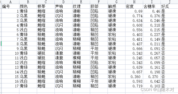
如上图所示的西瓜数据集,对测试样例编号1进行分类。对于先验概率
P
(
c
)
P(c)
P(c),有
P
(
好
瓜
=
是
)
=
8
17
P(好瓜=是)=\dfrac{8}{17}
P(好瓜=是)=178
P
(
好
瓜
=
否
)
=
9
17
P(好瓜=否)=\dfrac{9}{17}
P(好瓜=否)=179
然后为每个属性估计条件概率
P
(
x
i
∣
c
)
P(x_{i}|c)
P(xi∣c):
P
青
绿
∣
是
=
P
(
色
泽
=
青
绿
∣
好
瓜
=
是
)
=
3
8
P_{青绿|是}=P(色泽=青绿|好瓜=是)=\dfrac{3}{8}
P青绿∣是=P(色泽=青绿∣好瓜=是)=83
P
蜷
缩
∣
是
=
P
(
根
蒂
=
蜷
缩
∣
好
瓜
=
是
)
=
5
8
P_{蜷缩|是}=P(根蒂=蜷缩|好瓜=是)=\dfrac{5}{8}
P蜷缩∣是=P(根蒂=蜷缩∣好瓜=是)=85…
p
密
度
:
0.697
∣
是
=
p
(
密
度
=
0.697
∣
好
瓜
=
是
)
=
1
2
π
∗
0.129
e
x
p
(
−
(
0.697
−
0.574
)
2
2
∗
0.12
9
2
)
p_{密度:0.697|是}=p(密度=0.697|好瓜=是)=\dfrac{1}{\sqrt{2\pi}*0.129}exp(-\dfrac{(0.697-0.574)^{2}}{2*0.129^{2}})
p密度:0.697∣是=p(密度=0.697∣好瓜=是)=2π∗0.1291exp(−2∗0.1292(0.697−0.574)2)
其余属性条件概率略
最后,
     P


     (


     好


     瓜


     =


     是


     )


     ≈


     0.063


    P(好瓜=是)\approx 0.063


P(好瓜=是)≈0.063


     P


     (


     好


     瓜


     =


     否


     )


     ≈


     6.80


     ∗


     1


      0


       −


       5


    P(好瓜=否)\approx 6.80*10^{-5}


P(好瓜=否)≈6.80∗10−5
由于
     0.063


     >


     6.80


     ∗


     1


      0


       −


       5


    0.063>6.80*10^{-5}


0.063>6.80∗10−5因此将样例1判定为“好瓜”。
二、相关代码
1.数据处理
该数据集是我通过西瓜书上的西瓜数据集随机生成的10000条数据。需要的评论留言。
代码如下(示例):
import numpy as np
import pandas as pd
data=pd.read_csv("DataOrDocu/NewWatermelon2.csv",index_col=0)
attributes=data.columns
path="DataOrDocu/PosterProbDict.npy"
feature=data[:,:-1]
label=data[:,-1]
featureTrain,featureTest,labelTrain,labelTest=train_test_split(feature,label,train_size=0.7,random_state=10)
labelTrain=np.reshape(labelTrain,(labelTrain.shape[0],1))
labelTest=np.reshape(labelTest,(labelTest.shape[0],1))

dataTrain=np.concatenate((featureTrain,labelTrain),axis=1)
dataTrain=pd.DataFrame(dataTrain,columns=attributes,index=None)
dataTest=np.concatenate((featureTest,labelTest),axis=1)
dataTest=pd.DataFrame(dataTest,columns=attributes,index=None)
2.生成朴素贝叶斯表(字典)
逻辑很简单,即根据式(1.3),先计算《好瓜=是|否》的先验概率,即
P
(
好
瓜
=
是
)
P(好瓜=是)
P(好瓜=是)和
P
(
好
瓜
=
否
)
P(好瓜=否)
P(好瓜=否),并以字典形式返回。然后计算各种条件概率比如
P
(
色
泽
=
青
绿
∣
好
瓜
=
是
)
P(色泽=青绿|好瓜=是)
P(色泽=青绿∣好瓜=是)等等,如果是离散属性,那么保存
P
(
a
=
a
i
∣
好
瓜
=
是
o
r
否
)
P(a=a_{i}|好瓜=是or否)
P(a=ai∣好瓜=是or否)等一系列条件概率;如果是连续属性,那么保存
p
好
瓜
,
属
性
a
p_{好瓜,属性a}
p好瓜,属性a的均值和方差。最后,将生成的字典保存成npy文件,方便后续使用。
关于如何判断属性的连续或离散性
此外,有一个问题其中有一个函数,用于判断某个属性是离散属性还是连续属性,我考虑了2种方案,但实际上并不都是完美的逻辑,只是针对具体的数据集具有逻辑的相对完备性。一是判断数据是否为字符类型,一般字符类型将其判断为离散属性,其他判断为连续属性,但很容易在其他数据集上发现例外;二是计算某属性的所有数据集中包含的值的所有种类,如果种类数量<一定的范围,那么,我即认定为其为离散值,大于该范围的,认定其为连续值。但当遇到稀疏数据时,此类办法也会经常失效。
具体代码如下:
import numpy as np

defPosteriorProbDivided(data,attributes,label,path):
    priorProba={}
    length=data.shape[0]
    labelKinds=KindsGet(data,label)#获取标签的所有类别
    posterProbTable={}try:for i in labelKinds:
            dataTemp=data.loc[data[label]==i]
            tempLength=dataTemp.shape[0]
            tempPrior=tempLength/length
            priorProba.update({i:tempPrior})
            tempAttr ={}# 用于保存所有属性的条件概率for j in attributes:if IfDivideAttr(data,j):
                   tempPosterProb=DivCondiProba(data,j,length)
                   tempAttr.update({j:tempPosterProb})#将该属性的条件概率保存else:
                    averageVar=ContiCondiProba(data,j)#如果该属性是连续值,那么将该属性的平均值和方差求出,并保存
                    tempAttr.update({j:averageVar})
            posterProbTable.update({i:tempAttr})try:
            np.save(path,posterProbTable)except FileExistsError as error:print(error)return priorProba
    except IndexError as error:print(error)defIfDivideAttr(data,attribute):#第一种判断属性离散还是连续的函数
    values=np.unique(data[attribute]).shape[0]#获取某一属性的值的种类
    length=data.shape[0]if values!=0:if values<=length/10:#如果某一属性的取值数量小于等于总数据量的十分之一,即判定其为离散值returnTrueelse:returnFalsedefIfDivideAttr2(data,attribute):#第二种判断属性离散还是连续的函数returnnotisinstance(data[attribute],float)defKindsGet(data,attribute):#用于将离散属性的所有值返回if IfDivideAttr(data,attribute):
        values=np.unique(np.array(data[attribute]))return values
    returnNonedefDivCondiProba(data,attribute,length):#计算某一离散属性的条件概率
    tempAttrValues = KindsGet(data, attribute)
    tempPosterProb ={}# 用于保存某一属性的后验概率for k in tempAttrValues:
        tempAttrPoster = data.loc[data[attribute]== k].shape[0]/ length  # 计算出当某属性a的值为k时,其在标签c上的条件概率P(k|c),并将其压进列表
        tempPosterProb.update({k: tempAttrPoster})return tempPosterProb

defContiCondiProba(data,attribute):#计算某一连续属性的平均值和方差
    contiValue=data[attribute]
    contiValue=np.array(contiValue)
    average=np.average(contiValue)
    variance=np.var(contiValue)return average,variance
根据朴素贝叶斯表计算预测标签
针对某个数据的每一个属性对应的值,如果是离散属性,那么就从表中获取,如果是离散属性,那么就根据表中的均值和方差计算条件概率。但是区别于式(1.3),在程序中我对连乘做了一个取对数,防止指数爆炸(方正就是防止差距过大)。然后一个判断正确率的函数,单纯计算预测数据中的正确比例。
defPosteriorFind(data,posterProbTabel,priorProba):#用于计算某单个数据的最后标签
    posterValues=[]#用于保存每一个标签的后验概率
    bayesProba=0for label in posterProbTabel:for attribute in posterProbTabel[label]:# attrValue=list(attribute.keys())[0]      #取出字典键值对中的健if IfDivideAttr2(data,attribute):
                tempValue=np.log(posterProbTabel[label][attribute][data[attribute]])
                bayesProba+=tempValue
            else:
                averageVar=posterProbTabel[label][attribute]
                xi=data[attribute]
                average,variance=averageVar[0],averageVar[1]
                tempValue=1/(np.square(2*pi)*variance)*np.exp(-(xi-average)**2/2*variance**2)
                tempValue=np.log(tempValue)
                bayesProba+=tempValue
        labelKey=label      #取出label的key
        labelPrior=priorProba[labelKey]
        bayesProba+=np.log(labelPrior)#将该循环内的标签c所对应的先验概率加入其中
        posterValues.append(bayesProba)
        bayesProba=0

    posterDict=zip(posterValues,list(posterProbTabel.keys()))
    posterDict=dict(posterDict)
    bestValue=np.max(posterValues)
    bestLabel=posterDict[bestValue]return bestLabel

defAccCal(data,label,PosterProbaTabel,priorProba):
    length=data.shape[0]
    acc=0for i inrange(data.shape[0]):
        labelPre=PosteriorFind(data.loc[i],PosterProbaTabel,priorProba)if labelPre==data[label][i]:
            acc+=1
    ratio=acc/length
    return ratio
总结
使用随机生成的10000条数据,按照0.7训练集,0.3测试集的比例。最后的正确率大概是百分之四十几
之后又使用了一下鸢尾花的数据集
结果如下正确率是百分之三十一(可以说是很辣鸡了
最后附上sklearn的高斯贝叶斯和决策树跑鸢尾花的正确率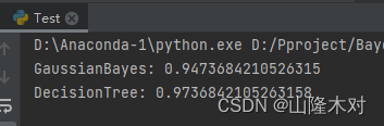
要不怎么说人家是专业的呢(doge
版权归原作者 山隆木对 所有, 如有侵权,请联系我们删除。