
优化器系列文章列表
Pytorch优化器全总结(一)SGD、ASGD、Rprop、Adagrad
Pytorch优化器全总结(二)Adadelta、RMSprop、Adam、Adamax、AdamW、NAdam、SparseAdam
Pytorch优化器全总结(三)牛顿法、BFGS、L-BFGS 含代码
Pytorch优化器全总结(四)常用优化器性能对比 含代码
写在前面
这篇文章是优化器系列的第三篇,主要介绍牛顿法、BFGS和L-BFGS,其中BFGS是拟牛顿法的一种,而L-BFGS是对BFGS的优化,那么事情还要从牛顿法开始说起。
一、牛顿法
函数最优化算法方法不唯一,其中耳熟能详的包括梯度下降法,梯度下降法是一种基于迭代的一阶优化方法,优点是计算简单;牛顿法也是一种很重要的优化方法,是基于迭代的二阶优化方法,优点是迭代次数少,收敛速度很快。下面我们简要介绍一下牛顿法。
1.看图理解牛顿法
最优化问题就是寻找能使函数最小化的x,所以目标函数应当是一个凸函数(起码是局部凸函数),假如一个函数如下图:
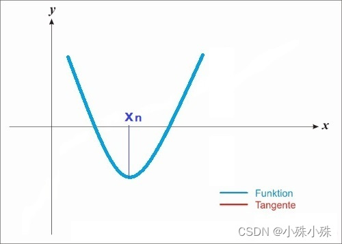
** 图1**
他的一阶导数可能长下面这个样子:
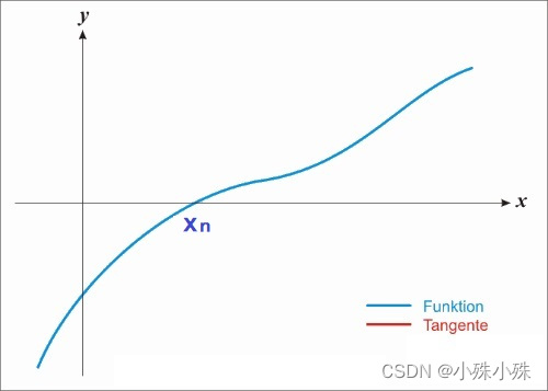
图2
很显然函数在处取得最小值,同时这个点的导数等于0,如果使用梯度下降,经过多次迭代,x的取值会慢慢接近,我们都能想象这个过程。
如果使用牛顿法,x也会逼近,不过速度会快很多,示例图如下:
图3
这个过程可以这样描述:
a.在X轴上随机一点,经过做X轴的垂线,得到垂线与函数图像的交点.
b.通过做函数的切线,得到切线与X轴的交点.
c.迭代a/b两步,当前后两次求的x相同或者两个值的差小于一个阈值的时候,我们就认为找到了。
三个步骤的难点在于b,如何快速的找到切线与X轴的交点,下面有两种计算方式,思想不同但结果是一样的。
2.公式推导-三角函数
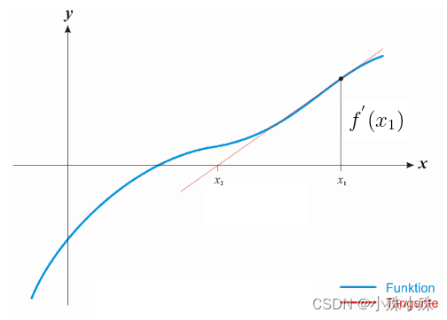
图4
如图4,蓝色的线是函数的的导数,则曲线在处的导数为,我们要求,根据三角函数有:
(1)
得出:
 (2)
利用开始进行下一轮的迭代。迭代公式可以简化如下:
(3)
3.公式推导-二阶泰勒展开
任意一点在附近的二阶泰勒展开公式为:
(4)
对求导:
(5)
令:
(6)
写成迭代形式:
(7)
可以看到使用三角函数和二阶泰勒展开最终得到的结果是一样的。虽然牛顿法收敛速度很快,但是当x的维度特别多的时候,我们想求得是非常困难的,而牛顿法又是一个迭代算法,所以这个困难我们还要面临无限多次,导致了直接使用牛顿法最为优化算法很难实际落地。为了解决这个问题出现了拟牛顿法,下面介绍一种拟牛顿法BFGS,主要就是想办法一种方法代替二阶导数。
二、BFGS公式推导
函数 在 处的二阶泰勒展开式为:
(8)
当x为向量的时候,上式写成:
(9)
令,同时对求导:
(10)
接下来我们要想办法去掉,我们使用代替,是在迭代中一点点计算出来的而不使用二阶导数。
上式变为:
(11)
(12)
我们认为每次迭代与上次变化,形式如下:
(13)
令:
,
(14)
将式(13)(14)带入式子(12):
(15)
令:
(16)
其中 均为 的向量,带入(15)
(17)
(18)
已知: 为实数, 为向量。式(18)中,参数 和 解的可能性有很多,我们取特殊的情况,假设 。带入(16)得:
(19)
将 带入(18)得:
(20)
(21)
令 ,则:
(22)
令,则
(23)
将式(22)和(23)带入(19):
(24)
将(24)带入(13)得到的迭代公式:
(24)
当x为向量的时候,式(7)写成:
(25)
加上学习率得到BFGS的迭代公式:
(26)
我们发现,还需要求的逆,这里可以引入sherman-morrism公式,求解的逆:
(27)
我们用代替,得到最终的BFGS迭代公式和的迭代公式:
(28)
(29)
其中是本轮x与上一轮x的差,是本轮梯度与上一轮梯度的差。
三、L-BFGS
在BFGS算法中,仍然有缺陷,每次迭代计算需要前次迭代得到的,的存储空间至少为N(N+1)/2(N为特征维数),对于高维的应用场景,需要的存储空间将是非常巨大的。为了解决这个问题,就有了L-BFGS算法。L-BFGS即Limited-memory BFGS。 L-BFGS的基本思想就是通过存储前m次迭代的少量数据来替代前一次的矩阵,从而大大减少数据的存储空间。
令,则式(29)可以表示为:
(30)
若在初始时,假定初始的矩阵,则我们可以得到:
(31)

 (32)


假设当前迭代为n,只保存最近的m次迭代信息,按照上面的方式迭代m次,可以得到如下的公式:


由于这些变量都最终可以由s、y两个向量计算得到,因此,我们只需存储最后m次的s、y向量即可算出,加上对角阵,总共需要存储2*m+1个N维向量(实际应用中m一般取4到7之间的值,因此需要存储的数据远小于Hesse矩阵)。
四、算法迭代过程
1. 选初始点,最小梯度阈值,存储最近 m 次的选代数据;
2.初始化;
3.如果,则返回最优解 x,否则转入步骤4;
4.计算本次选代的可行方向;
5.计算步长,用下面的式子进行线搜索;
6.用下面的更新公式更新x;
7.如果 n大于 m,保留最近 m 次的向量对,删除;
8.计算并保存向量对
9.用 two-loop recursion算法求:
10.设置,转到步骤3
五、代码实现
1.torch.optim.LBFGS说明
    该类实现 LBFGS优化方法。LBFGS是什么已经不用多说了。

    Pytorch说明文档:LBFGS — PyTorch 1.13 documentation
'''
lr (float): 学习率 (default: 1)
max_iter (int): 每个优化步骤的最大迭代次数,就像图3那样迭代 (default: 20)
max_eval (int): 每次优化函数计算的最大数量,使用了线搜索算法时,每次迭代计数器可能增加不止1,最好使用线搜索算法时再设置这个参数。计数器同时受max_iter 和max_eval约束,先到哪个值直接跳出迭代。(default: max_iter * 1.25).
tolerance_grad (float): 一阶最优终止公差,就是指yn (default: 1e-5).
tolerance_change (float): 函数值/参数变化的终止容差,就是指sn (default: 1e-9).
history_size (int): 更新历史记录大小 (default: 100).
line_search_fn (str): 使用线搜索算法,只能是'strong_wolfe' 或者None (default: None).
'''
class torch.optim.LBFGS(params, lr=1.0, rho=0.9, eps=1e-06, weight_decay=0)
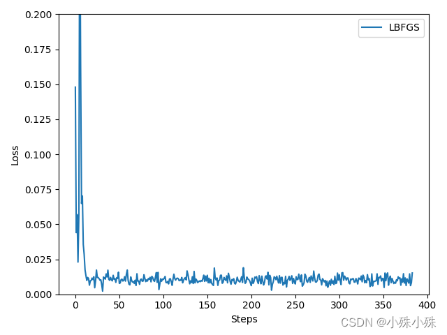
2.使用LBFGS优化模型
我们用一个简单的全连接网络并使用LBFGS优化,下面是代码和运行结果,可以看到,损失下降的速度还是很快的。
# coding=utf-8
#================================================================
#
#   File name   : optim_duibi.py
#   Author      : Faye
#   Created date: 2022/8/26 17:30
#   Description :
#
#================================================================

import torch
import torch.utils.data as Data
import torch.nn.functional as F
from torch.autograd import Variable
import matplotlib.pyplot as plt

# 超参数
LR = 0.01
BATCH_SIZE = 32
EPOCH = 12

# 生成假数据
# torch.unsqueeze() 的作用是将一维变二维,torch只能处理二维的数据
x = torch.unsqueeze(torch.linspace(-1, 1, 1000), dim=1)  # x data (tensor), shape(100, 1)
# 0.2 * torch.rand(x.size())增加噪点
y = x.pow(2) + 0.1 * torch.normal(torch.zeros(*x.size()))

# 定义数据库
dataset = Data.TensorDataset(x, y)

# 定义数据加载器
loader = Data.DataLoader(dataset=dataset, batch_size=BATCH_SIZE, shuffle=True, num_workers=0)

# 定义pytorch网络
class Net(torch.nn.Module):
    def __init__(self, n_features, n_hidden, n_output):
        super(Net, self).__init__()
        self.hidden = torch.nn.Linear(n_features, n_hidden)
        self.predict = torch.nn.Linear(n_hidden, n_output)

    def forward(self, x):
        x = F.relu(self.hidden(x))
        y = self.predict(x)
        return y

# 定义不同的优化器网络
net_LBFGS = Net(1, 10, 1)

# 选择不同的优化方法
opt_LBFGS = torch.optim.LBFGS(net_LBFGS.parameters(), lr=LR, max_iter=20)

nets = [net_LBFGS]
optimizers = [opt_LBFGS]

# 选择损失函数
loss_func = torch.nn.MSELoss()

# 不同方法的loss
loss_LBFGS = []

# 保存所有loss
losses = [loss_LBFGS]

# 执行训练
for epoch in range(EPOCH):
    for step, (batch_x, batch_y) in enumerate(loader):
        var_x = Variable(batch_x)
        var_y = Variable(batch_y)
        for net, optimizer, loss_history in zip(nets, optimizers, losses):
            if isinstance(optimizer, torch.optim.LBFGS):
                def closure():
                    y_pred = net(var_x)
                    loss = loss_func(y_pred, var_y)
                    optimizer.zero_grad()
                    loss.backward()
                    return loss
                loss = optimizer.step(closure)
            else:
                # 对x进行预测
                prediction = net(var_x)
                # 计算损失
                loss = loss_func(prediction, var_y)
                # 每次迭代清空上一次的梯度
                optimizer.zero_grad()
                # 反向传播
                loss.backward()
                # 更新梯度
                optimizer.step()
            # 保存loss记录
            loss_history.append(loss.data)

# 画图
labels = ['LBFGS']
for i, loss_history in enumerate(losses):
    plt.plot(loss_history, label=labels[i])
plt.legend(loc='best')
plt.xlabel('Steps')
plt.ylabel('Loss')
plt.ylim((0, 0.2))
plt.show()
牛顿法、BFGS和L-BFGS就介绍到这里,后面我将对比所有优化算法的性能,收藏关注不迷路。
优化器系列文章列表
Pytorch优化器全总结(一)SGD、ASGD、Rprop、Adagrad
Pytorch优化器全总结(二)Adadelta、RMSprop、Adam、Adamax、AdamW、NAdam、SparseAdam
Pytorch优化器全总结(三)牛顿法、BFGS、L-BFGS 含代码
Pytorch优化器全总结(四)常用优化器性能对比 含代码
版权归原作者 小殊小殊 所有, 如有侵权,请联系我们删除。