
通过细胞图像的标签对模型性能的影响,为数据设置优先级和权重。
许多机器学习任务的主要障碍之一是缺乏标记数据。而标记数据可能会耗费很长的时间,并且很昂贵,因此很多时候尝试使用机器学习方法来解决问题是不合理的。
为了解决这个问题,机器学习领域出现了一个叫做主动学习的领域。主动学习是机器学习中的一种方法,它提供了一个框架,根据模型已经看到的标记数据对未标记的数据样本进行优先排序。如果想
细胞成像的分割和分类等技术是一个快速发展的领域研究。就像在其他机器学习领域一样,数据的标注是非常昂贵的,并且对于数据标注的质量要求也非常的高。针对这一问题,本篇文章介绍一种对红细胞和白细胞图像分类任务的主动学习端到端工作流程。
我们的目标是将生物学和主动学习的结合,并帮助其他人使用主动学习方法解决生物学领域中类似的和更复杂的任务。
本篇文主要由三个部分组成:
- 细胞图像预处理——在这里将介绍如何预处理未分割的血细胞图像。
- 使用CellProfiler提取细胞特征——展示如何从生物细胞照片图像中提取形态学特征,以用作机器学习模型的特征。
- 使用主动学习——展示一个模拟使用主动学习和不使用主动学习的对比实验。
细胞图像预处理
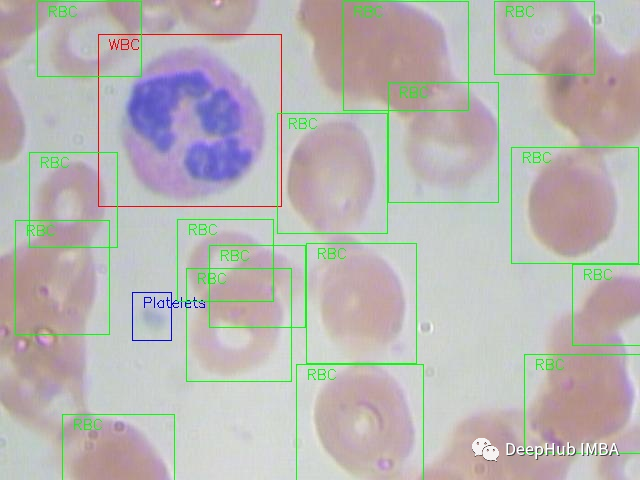
我们将使用在MIT许可的血细胞图像数据集(GitHub和Kaggle)。每张图片都根据红细胞(RBC)和白细胞(WBC)分类进行标记。对于这4种白细胞(嗜酸性粒细胞、淋巴细胞、单核细胞和中性粒细胞)还有附加的标签,但在本文的研究中没有使用这些标签。
下面是一个来自数据集的全尺寸原始图像的例子:
创建样本DF
原始数据集包含一个export.py脚本,它将XML注释解析为一个CSV表,其中包含每个细胞的文件名、细胞类型标签和边界框。
原始脚本没有包含cell_id列,但我们要对单个细胞进行分类,所以我们稍微修改了代码,添加了该列并添加了一列包括image_id和cell_id的filename列:
import os, sys, random
import xml.etree.ElementTree as ET
from glob import glob
import pandas as pd
from shutil import copyfile

annotations = glob('BCCD_Dataset/BCCD/Annotations/*.xml')
df = []
for file in annotations:
    #filename = file.split('/')[-1].split('.')[0] + '.jpg'
    #filename = str(cnt) + '.jpg'
    filename = file.split('\\')[-1]
    filename =filename.split('.')[0] + '.jpg'
    row = []
    parsedXML = ET.parse(file)
    cell_id = 0
    for node in parsedXML.getroot().iter('object'):
        blood_cells = node.find('name').text
        xmin = int(node.find('bndbox/xmin').text)
        xmax = int(node.find('bndbox/xmax').text)
        ymin = int(node.find('bndbox/ymin').text)
        ymax = int(node.find('bndbox/ymax').text)

        row = [filename, cell_id, blood_cells, xmin, xmax, ymin, ymax]
        df.append(row)
        cell_id += 1

data = pd.DataFrame(df, columns=['filename', 'cell_id', 'cell_type', 'xmin', 'xmax', 'ymin', 'ymax'])
data['image_id'] = data['filename'].apply(lambda x: int(x[-7:-4]))
data[['filename', 'image_id', 'cell_id', 'cell_type', 'xmin', 'xmax', 'ymin', 'ymax']].to_csv('bccd.csv', index=False)
裁剪
为了能够处理数据,第一步是根据边界框坐标裁剪全尺寸图像。这就产生了很多大小不一的细胞图像:
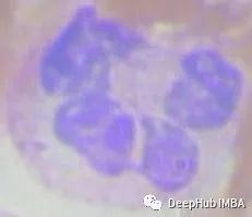


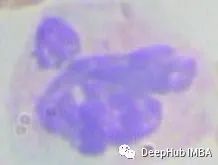
裁剪的代码如下:
import os
import pandas as pd
from PIL import Image

def crop_cell(row):
    """
    crop_cell(row)

    given a pd.Series row of the dataframe, load row['filename'] with PIL,
    crop it to the box row['xmin'], row['xmax'], row['ymin'], row['ymax']
    save the cropped image,
    return cropped filename
    """
    input_dir = 'BCCD\JPEGImages'
    output_dir = 'BCCD\cropped'
    # open image
    im = Image.open(f"{input_dir}\{row['filename']}")

    # size of the image in pixels
    width, height = im.size

    # setting the points for cropped image
    left = row['xmin']
    bottom = row['ymax']
    right = row['xmax']
    top = row['ymin']

    # cropped image
    im1 = im.crop((left, top, right, bottom))
    cropped_fname = f"BloodImage_{row['image_id']:03d}_{row['cell_id']:02d}.jpg"
    # shows the image in image viewer
    # im1.show()

    # save image
    try:
        im1.save(f"{output_dir}\{cropped_fname}")
    except:
        return 'error while saving image'

    return cropped_fname

if __name__ == "__main__":
    # load labels csv into Pandas DataFrame
    filepath = "BCCD\dataset2-master\labels.csv"
    df = pd.read_csv(filepath)

    # iterate through cells, crop each cell, and save cropped cell to file
    dataset_df['cell_filename'] = dataset_df.apply(crop_cell, axis=1)
以上就是我们所做的所有预处理操作。现在,我们继续使用CellProfiler提取特征。
使用CellProfiler提取细胞特征
CellProfiler是一个免费的开源图像分析软件,可以从大规模细胞图像中自动定量测量。CellProfiler还包含一个GUI界面,允许我们可视化的操作
首先下载CellProfiler,如果CellProfiler无法打开,则可能需要安装Visual C ++发布包,具体安装方式参考官网。
打开软件就可以加载图像了, 如果想构建管道可以在CellProfiler官网找到其提供的可用的功能列表。大多数功能分为三个主要组:图像处理,目标的处理和测量。
常用的功能如下:
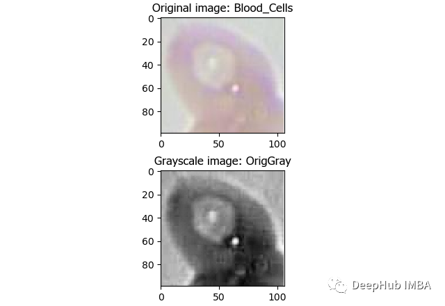
图像处理 - 转为灰度图:
目标对象处理 - 识别主要对象
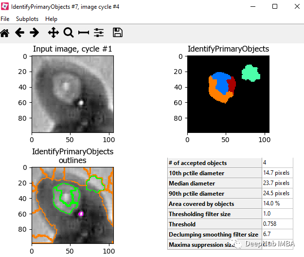
测量 - 测量对象强度
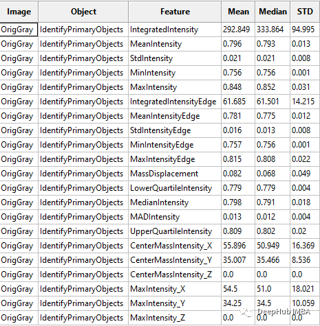
CellProfiler可以将输出为CSV文件或者保存指定数据库中。这里我们将输出保存为CSV文件,然后将其加载到Python进行进一步处理。
说明:CellProfiler还可以将你处理图像的流程保存并进行分享。
主动学习
我们现在已经有了训练需要的搜有数据,现在可以开始试验使用主动学习策略是否可以通过更少的数据标记获得更高的准确性。我们的假设是:使用主动学习可以通过大量减少在细胞分类任务上训练机器学习模型所需的标记数据量来节省宝贵的时间和精力。
主动学习框架
在深入研究实验之前,我们希望对modAL进行快速介绍:modAL是Python的活跃学习框架。它提供了Sklearn API,因此可以非常容易的将其集成到代码中。该框架可以轻松地使用不同的主动学习策略。他们的文档也很清晰,所以建议从它开始你的一个主动学习项目。
主动学习与随机学习
为了验证假设,我们将进行一项实验,将添加新标签数据的随机子抽样策略与主动学习策略进行比较。开始用一些相同的标记样本训练2个Logistic回归估计器。然后将在一个模型中使用随机策略,在第二个模型中使用主动学习策略。
我们首先为实验准备数据,加载由Cell Profiler创建的特征。这里过滤了无色血细胞的血小板,只保留红和白细胞(将问题简化,并减少数据量) 。所以现在我们正在尝试解决二进制分类问题 - RBC与WBC。使用Sklearn Label的label encoder进行编码,并拆分数据集进行训练和测试。
# imports for the whole experiment
import numpy as np
from matplotlib import pyplot as plt
from modAL import ActiveLearner
import pandas as pd
from modAL.uncertainty import uncertainty_sampling
from sklearn import  preprocessing
from sklearn.metrics import , average_precision_score
from sklearn.linear_model import LogisticRegression

# upload the cell profiler features for each cell
data = pd.read_csv('Zaretski_Image_All.csv')

# filter platelets
data = data[data['cell_type'] != 'Platelets']

# define the label
target = 'cell_type'
label_encoder = preprocessing.LabelEncoder()
y = label_encoder.fit_transform(data[target])

# take the learning features only
X = data.iloc[:, 5:]

# create training and testing sets
X_train, X_test, y_train, y_test = train_test_split(X.to_numpy(), y, test_size=0.33, random_state=42)
下一步就是创建模型
dummy_learner = LogisticRegression()

active_learner = ActiveLearner(
  estimator=LogisticRegression(),
  query_strategy=uncertainty_sampling()
)
dummy_learner是使用随机策略的模型,而active_learner是使用主动学习策略的模型。为了实例化一个主动学习模型,我们使用modAL包中的ActiveLearner对象。在“estimator”字段中,可以插入任何sklearnAPI兼容的模型。在query_strategy '字段中可以选择特定的主动学习策略。这里使用“uncertainty_sampling()”。这方面更多的信息请查看modAL文档。
将训练数据分成两组。第一个是训练数据,我们知道它的标签,会用它来训练模型。第二个是验证数据,虽然标签也是已知的但是我们假装不知道它的标签,并通过模型预测的标签和实际标签进行比较来评估模型的性能。然后我们将训练的数据样本数设置成5。
# the training size that we will start with
base_size = 5

# the 'base' data that will be the training set for our model
X_train_base_dummy = X_train[:base_size]
X_train_base_active = X_train[:base_size]
y_train_base_dummy = y_train[:base_size]
y_train_base_active = y_train[:base_size]

# the 'new' data that will simulate unlabeled data that we pick a sample from and label it
X_train_new_dummy = X_train[base_size:]
X_train_new_active = X_train[base_size:]
y_train_new_dummy = y_train[base_size:]
y_train_new_active = y_train[base_size:]
我们训练298个epoch,在每个epoch中,将训练这俩个模型和选择下一个样本,并根据每个模型的策略选择是否将样本加入到我们的“基础”数据中,并在每个epoch中测试其准确性。因为分类是不平衡的,所以使用平均精度评分来衡量模型的性能。
在随机策略中选择下一个样本,只需将下一个样本添加到虚拟数据集的“新”组中,这是因为数据集已经是打乱的的,因此不需要再进行这个操作。对于主动学习,将使用名为“query”的ActiveLearner方法,该方法获取“新”组的未标记数据,并返回他建议添加到训练“基础”组的样本索引。被选择的样本都将从组中删除,因此样本只能被选择一次。
# arrays to accumulate the scores of each simulation along the epochs
dummy_scores = []
active_scores = []
# number of desired epochs
range_epoch = 298
# running the experiment
for i in range(range_epoch):
   # train the models on the 'base' dataset
   active_learner.fit(X_train_base_active, y_train_base_active)
   dummy_learner.fit(X_train_base_dummy, y_train_base_dummy)

   # evaluate the models
   dummy_pred = dummy_learner.predict(X_test)
   active_pred = active_learner.predict(X_test)

   # accumulate the scores
   dummy_scores.append(average_precision_score(dummy_pred, y_test))
   active_scores.append(average_precision_score(active_pred, y_test))

   # pick the next sample in the random strategy and randomly
   # add it to the 'base' dataset of the dummy learner and remove it from the 'new' dataset
   X_train_base_dummy = np.append(X_train_base_dummy, [X_train_new_dummy[0, :]], axis=0)
   y_train_base_dummy = np.concatenate([y_train_base_dummy, np.array([y_train_new_dummy[0]])], axis=0)
   X_train_new_dummy = X_train_new_dummy[1:]
   y_train_new_dummy = y_train_new_dummy[1:]

   # pick next sample in the active strategy
   query_idx, query_sample = active_learner.query(X_train_new_active)

   # add the index to the 'base' dataset of the active learner and remove it from the 'new' dataset
   X_train_base_active = np.append(X_train_base_active, X_train_new_active[query_idx], axis=0)
   y_train_base_active = np.concatenate([y_train_base_active, y_train_new_active[query_idx]], axis=0)
   X_train_new_active = np.concatenate([X_train_new_active[:query_idx[0]], X_train_new_active[query_idx[0] + 1:]], axis=0)
   y_train_new_active = np.concatenate([y_train_new_active[:query_idx[0]], y_train_new_active[query_idx[0] + 1:]], axis=0)
结果如下:
plt.plot(list(range(range_epoch)), active_scores, label='Active Learning')
plt.plot(list(range(range_epoch)), dummy_scores, label='Dummy')
plt.xlabel('number of added samples')
plt.ylabel('average precision score')
plt.legend(loc='lower right')
plt.savefig("models robustness vs dummy.png", bbox_inches='tight')
plt.show()
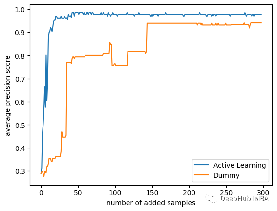
策略之间的差异还是很大的,可以看到主动学习只使用25个样本就可以达到平均精度0.9得分!而使用随机的策略则需要175个样本才能达到相同的精度!
此外主动学习策略的模型的分数接近0.99,而随机模型的分数在0.95左右停止了!如果我们使用所有数据,那么它们最终分数是相同的,但是我们的研究目的是在少量标注数据的前提下训练,所以只使用了数据集中的300个随机样本。
总结
本文展示了将主动学习用于细胞成像任务的好处。主动学习是机器学习中的一组方法,可根据其标签对模型性能的影响来优先考虑未标记的数据示例的解决方案。由于标记数据是一项涉及许多资源(金钱和时间)的任务,因此判断那些标记那些样本可以最大程度地提高模型的性能是非常必要的。
细胞成像为生物学,医学和药理学领域做出了巨大贡献。以前分析细胞图像需要有价值的专业人力资本,但是像主动学习这种技术的出现为医学领域这种需要大量人力标注数据集的领域提供了一个非常好的解决方案。s
本文引用:
- GitHub — Shenggan/BCCD_Dataset: BCCD (Blood Cell Count and Detection) Dataset is a small-scale dataset for blood cells detection.
- Blood Cell Images | Kaggle
- Active Learning in Machine Learning | by Ana Solaguren-Beascoa, PhD | Towards Data Science
- Carpenter, A. E., Jones, T. R., Lamprecht, M. R., Clarke, C., Kang, I. H., Friman, O., … & Sabatini, D. M. (2006).
- CellProfiler: image analysis software for identifying and quantifying cell phenotypes. Genome biology, 7(10), 1–11.
- Stirling, D. R., Swain-Bowden, M. J., Lucas, A. M., Carpenter, A. E., Cimini, B. A., & Goodman, A. (2021).
作者:Adi Nissim, Noam Siegel, Nimrod Berman