动手学习ResNet50

ResNet 论文

《Deep Residual Learning for Image Recognition》
论文地址：https://arxiv.org/abs/1512.03385

残差网络(ResNet)

以学习ResNet的收获、ResNet50的复现二大部分，简述ResNet50网络。

一、学习ResNet的收获

1. ResNet网络解决了深度CNN模型难训练的问题，并指出CNN模型随深度的加深可以得到更优的解，对于 plain/residual nets 均如此。随着 nets的加深，plain nets 的收敛速度变得缓慢，导致了CNN模型的深层网络不如较浅层网络，但是 residual nets 解决了这个问题。至于 residual nets 如何解决深层网络收敛速度变得缓慢的问题，得益于 residual learning 。
2. Residual learning 的理想公式为 F ( x ) = H ( x ) − x . ( 1 ) F(x) = H(x)-x.(1) F(x)=H(x)−x.(1) H ( x ) = F ( x ) + x . ( 2 ) H(x)=F(x)+x.(2) H(x)=F(x)+x.(2) 设所需求解的底层映射为H(x)，通过训练堆叠的非线性层映射F(x)=H(x)-x，因此H(x)=F(x)+x。 但是 Residual learning 的实际使用公式为 y = F ( x , W i ) + x . ( 3 ) y=F(x,\mathop{W}{i})+x.(3) y=F(x,Wi​)+x.(3) 或 y = F ( x , W i ) + W s x . ( 4 ) 或y=F(x,\mathop{W}{i})+\mathop{W}_{s}x.(4) 或y=F(x,Wi​)+Ws​x.(4) 设x、y、F分别为输入、输出、堆叠的非线性层映射。采用标识性快捷连接(Identity Mapping by Shortcuts)，把输入x与堆叠的非线性层映射F相加得到输出y。其中Wi,Ws均为线性投影，对于x和F的维数（及尺寸），相同时使用公式(3)，不相同时使用公式(4)。 （Fig 2.为 Residual learning 的结构图）
3. 对于 plain/residual nets 的深度探究与验证。1). plain nets 随着网络深度的加深，plain nets 的性能降低并非由梯度消失或梯度爆炸引起。对于 20-layer and 56-layer “plain” networks，其 training error 和 test error 随网络深度的加深而提高，但并非无法训练(如Fig 1.)。因此网络深度的加深，导致了网络收敛速度的降低。2). residual nets 随着网络深度的加深，residual nets 的性能提升并非一成不变。《Deep Residual Learning for Image Recognition》指出 1202-layers ResNet 的 error 比 110-layers ResNet 的 error 高出 1.5% 左右，在CIFAR-10数据集及其他条件相同下测得(见 Table 6.)。何博士猜测数据集的规模未能匹配网络的规模，造成 residual nets 性能的降低（通俗：数据集的规模太小而网络的深度太大，造成 residual nets 性能的降低）。

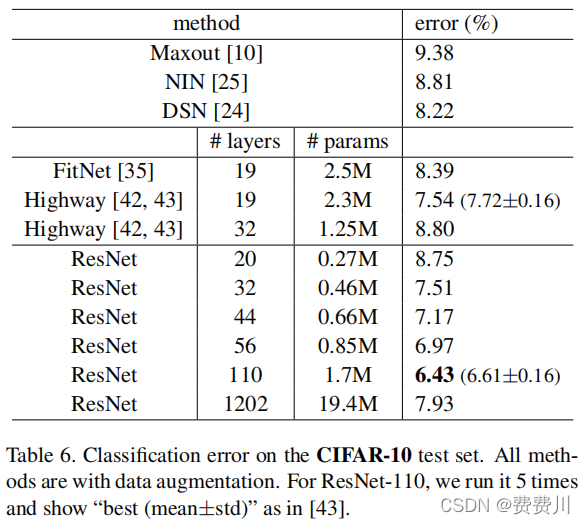
二、ResNet50的复现

通过九大部分复现ResNet50，例如数据增强、参数控制、数据集构建、网络构建、模型加载、模型训练、绘制损失图、模型验证、模型预测。

1. 数据增强

    数据增强由缩放、裁剪、旋转、亮度、对比度、颜色的变化组成。调用pytorch的     transformer完成。
    注意transformer匹配PIL的RGB格式，而非Opencv的BGR格式。

打开图片

import matplotlib.pyplot as plt
from PIL import Image
from torchvision import transforms as tfs

img = Image.open('gift/bald3.jpg')
plt.imshow(img)
plt.show()# print(img.size)--->(301, 301)

比例缩放

# 比例缩放# rint('before scale, shape:{}'.format(img.size))-->(before scale, shape:(301, 301))# 参数为元组(row,col)时,图片尺寸硬性放缩为(row,col)(宽,长)# 参数为数字size时，图片按比例缩放，其中min(row,col)=size
new_img = tfs.Resize(256)(img)# print('after scale, shape:{}'.format(new_img.size))-->(after scale, shape:(256, 256))
plt.imshow(new_img)
plt.show()

随机裁剪

# 随机裁剪
random_img = tfs.RandomCrop(224)(new_img)
plt.imshow(random_img)
plt.show()

随机旋转

# 随机角度旋转for i inrange(1):
    rot_img = tfs.RandomRotation(180)(new_img)
    plt.imshow(rot_img)
    plt.show()

# 在这里给出图片翻转的代码，效果自行实验# 随机水平翻转
h_filp = tfs.RandomHorizontalFlip()(new_img)
plt.imshow(h_filp)
plt.show()# 随机竖直翻转
v_filp = tfs.RandomVerticalFlip()(new_img)
plt.imshow(v_filp)
plt.show()

亮度变化

# 亮度
bright_img = tfs.ColorJitter(brightness=1)(new_img)# 随机从 0---2 之间亮度变化，1 表示原图
plt.imshow(bright_img)
plt.show()

对比度变化

# 对比度
contrast_img = tfs.ColorJitter(contrast=1)(new_img)# 随机从 0---2 之间对比度变化，1 表示原图
plt.imshow(contrast_img)
plt.show()

颜色变化

# 颜色
color_img = tfs.ColorJitter(hue=0.5)(new_img)# 随机从 -0.5---0.5 之间对颜色变化
plt.imshow(color_img)
plt.show()

数据增强总实验

img_aug = tfs.Compose([
    tfs.Resize(256),
    tfs.RandomRotation(180),
    tfs.RandomCrop(224),
    tfs.ColorJitter(brightness=0.5, contrast=0.5, hue=0.5)])# 以九宫格的形式展示
nrows =3
ncols =3
figsize =(32,32)
_, figs = plt.subplots(nrows, ncols, figsize=figsize)for i inrange(nrows):for j inrange(ncols):
        figs[i][j].imshow(img_aug(img))
        figs[i][j].axes.get_xaxis().set_visible(False)
        figs[i][j].axes.get_yaxis().set_visible(False)
plt.show()

2. 参数控制

batch_size =32# 每次喂入的数据量
lr         =0.01# 学习率
step_size  =1# 每n个epoch更新一次学习率
epoch_num  =10# 总迭代次数
num_print  =280# 每n次batch打印一次
num_check  =1# 每n个epoch验证一次模型，若效果更优则保存模型
enhance    =False# 是否数据增强

3. 数据集构建

数据预处理，采用标准化处理。详细见动手学习VGG16的数据预处理。

"""
train_path、verification_path、test_path 同为字典（类别kind，列表list），其中列表内存放着图片的绝对路径。
labels 也是一个字典（类别kind，序号number），序号为1~n的数字
"""import torch
import random
from PIL import Image
from torch.autograd import Variable
from torchvision import transforms
from torch.utils.data import Dataset, DataLoader

en_transform = transforms.Compose([
    transforms.Resize(256),
    transforms.RandomRotation(180),
    transforms.RandomCrop(224),
    transforms.ColorJitter(brightness=0.5, contrast=0.5, hue=0.5),
    transforms.ToTensor(),
    transforms.Normalize((0.51865010496974,0.49877608954906466,0.5143190141916275),(7.181780141103533,8.053991771959863,8.290017965464534))])

no_transform = transforms.Compose([
    transforms.Resize(224),
    transforms.ToTensor(),
    transforms.Normalize((0.51865010496974,0.49877608954906466,0.5143190141916275),(7.181780141103533,8.053991771959863,8.290017965464534))])# -----------------ready the dataset--------------------------defdefault_loader(path):
    img = Image.open(path)return img

classMyDataset(Dataset):# 构造函数def__init__(self, path, transform=None, target_transform=None, loader=default_loader, enhance=False):
        imgs =[]for classification in path:for i inrange(len(path[classification])):
                img_path  = path[classification][i]
                img_label = labels[classification]
                imgs.append((img_path,int(img_label)))#imgs中包含有图像路径和标签
        self.path             = path
        self.imgs             = imgs
        self.transform        = transform
        self.target_transform = target_transform
        self.loader           = loader
        
    # hash_map建立def__getitem__(self, index):
        img_path, img_label = self.imgs[index]# 调用 opencv 打开图片
        img = self.loader(img_path)if self.transform isnotNone:
            img = self.transform(img)
        img_label -=1return img, img_label
    
    def__len__(self):returnlen(self.imgs)

train_data        = MyDataset(train_path, transform=no_transform,target_transform=en_transform,enhance=True)
verification_data = MyDataset(verification_path, transform=no_transform,target_transform=en_transform,enhance=False)
test_data         = MyDataset(test_path, transform=no_transform,target_transform=en_transform,enhance=False)#train_data 、verification_data和test_data包含多有的训练、验证与测试数据，调用DataLoader批量加载
train_loader        = DataLoader(dataset=train_data, batch_size=batch_size, shuffle=True)
verification_loader = DataLoader(dataset=verification_data, batch_size=batch_size, shuffle=False)
test_loader         = DataLoader(dataset=test_data, batch_size=batch_size, shuffle=False)

4. 网络构建

ResNet网络由数个残差块及卷积层构成，残差块的结构决定了ResNets。在这里给出何博士提到的2个结构分别为original、proposed,其中original为论文的主要实验对象，proposed为何博士于附录中提及。(其结构及性能见图8）参考于你必须要知道CNN模型：ResNet。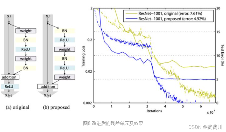

import torch
from torch import optim
import torchvision
import matplotlib.pyplot as plt
import numpy as np
from torchvision.utils import make_grid
import time
from torch import nn
from torchsummary import summary

残差块-original

# 残差块classResidual(nn.Module):def__init__(self,input_channels, temp_channels, num_channels,
                  use_1x1conv=False, strides=1):super(Residual, self).__init__()
        
        self.conv1 = nn.Conv2d(input_channels, temp_channels,
                                   kernel_size=1, stride=strides)
        self.conv2 = nn.Conv2d(temp_channels, temp_channels,
                                   kernel_size=3, padding=1)
        self.conv3 = nn.Conv2d(temp_channels, num_channels,
                                   kernel_size=1)if use_1x1conv:
            self.conv4 = nn.Conv2d(input_channels,num_channels,
                                   kernel_size=1,stride=strides)else:
            self.conv4 =None
                
        self.bn1 = nn.BatchNorm2d(temp_channels)
        self.bn2 = nn.BatchNorm2d(temp_channels)
        self.bn3 = nn.BatchNorm2d(num_channels)
        
        self.rl1 = nn.ReLU(inplace=True)
        self.rl2 = nn.ReLU(inplace=True)
        self.rl3 = nn.ReLU(inplace=True)defforward(self, x):
        y = self.rl1(self.bn1(self.conv1(x)))
        y = self.rl2(self.bn2(self.conv2(y)))
        y = self.bn3(self.conv3(y))if self.conv4:
            x = self.conv4(x)return self.rl3(y + x)

残差块-proposed

# 残差块classResidual(nn.Module):def__init__(self,input_channels, temp_channels, num_channels,
                  use_1x1conv=False, strides=1):super(Residual, self).__init__()
        
        self.conv1 = nn.Conv2d(input_channels, temp_channels,
                                   kernel_size=1, stride=strides)
        self.conv2 = nn.Conv2d(temp_channels, temp_channels,
                                   kernel_size=3, padding=1)
        self.conv3 = nn.Conv2d(temp_channels, num_channels,
                                   kernel_size=1)if use_1x1conv:
            self.conv4 = nn.Conv2d(input_channels,num_channels,
                                   kernel_size=1,stride=strides)else:
            self.conv4 =None
                
        self.bn1 = nn.BatchNorm2d(input_channels)
        self.bn2 = nn.BatchNorm2d(temp_channels)
        self.bn3 = nn.BatchNorm2d(temp_channels)
        
        self.rl1 = nn.ReLU(inplace=True)
        self.rl2 = nn.ReLU(inplace=True)
        self.rl3 = nn.ReLU(inplace=True)defforward(self, x):
        y = self.conv1(self.rl1(self.bn1(x)))
        y = self.conv2(self.rl2(self.bn2(y)))
        y = self.conv3(self.rl3(self.bn3(y)))if self.conv4:
            x = self.conv4(x)return y + x

ResNet50网络

# 残差网络# Residual封装defresent_block(channels, num_residuals, first_block=False):
    blk =[]
    input_channels, temp_channels, num_channels = channels
    for i inrange(num_residuals):if i ==0and first_block:
            blk.append(Residual(channels[0], channels[1], channels[2],
                                use_1x1conv=True))elif i ==0andnot first_block:
            blk.append(Residual(channels[0], channels[1], channels[2],
                                use_1x1conv=True, strides=2))else:
            blk.append(Residual(channels[2], channels[1], channels[2]))return blk

# ResNet50定义classResNet50(nn.Module):def__init__(self):super(ResNet50, self).__init__()# 第一层，1个卷积层和1个最大池化层
        self.layer1 = nn.Sequential(
            nn.Conv2d(3,64, kernel_size=7, stride=2, padding=3),
            nn.BatchNorm2d(64),
            nn.ReLU(inplace=True),
            
            nn.MaxPool2d(kernel_size=3, stride=2, padding=1))# 第二层，3 * 3个卷积层
        self.layer2 = nn.Sequential(*resent_block((64,64,256),3, first_block=True))# 第三层，4 * 3个卷积层
        self.layer3 = nn.Sequential(*resent_block((256,128,512),4))# 第四层，6 * 3个卷积层
        self.layer4 = nn.Sequential(*resent_block((512,256,1024),6))# 第五层，3 * 3个卷积层
        self.layer5 = nn.Sequential(*resent_block((1024,512,2048),3))
        
        self.conv_layer = nn.Sequential(
            self.layer1,
            self.layer2,
            self.layer3,
            self.layer4,
            self.layer5
        )
        
        self.fc = nn.Sequential(
            nn.Linear(2048,1000),
            nn.ReLU(inplace=True),
            
            nn.Linear(1000,29))defforward(self, x):
        x = self.conv_layer(x)# 全局平均池化层
        x = nn.functional.adaptive_avg_pool2d(x,(1,1))
        x = x.view(x.size(0),-1)
        x = self.fc(x)return x

# 验证网络是否可运行if __name__ =="__main__":
    device       = torch.device('cuda'if torch.cuda.is_available()else'cpu')
    resent_model = ResNet50().to(device)
    summary(resent_model,(3,224,224))#打印网络结构

其中original、proposed结构的ResNet50的参数均为18kw，区别于卷积层、归一化层、激活函数ReLU层的顺序不同。

5. 模型加载

# ResNet50
PATH   =Noneifnot PATH:
    device      = torch.device("cuda:0"if torch.cuda.is_available()else"cpu")
    model       = ResNet50().to(device)else:
    model  = ResNet50()
    model.load_state_dict(torch.load(PATH), strict=False)
    model.eval()
    device = torch.device("cuda:0"if torch.cuda.is_available()else"cpu")
    model.to(device)
    summary(model,(3,224,224))# 调参# 交叉熵
criterion = nn.CrossEntropyLoss()# 迭代器
optimizer = optim.SGD(model.parameters(), lr=lr, momentum=0.8, weight_decay=0.001)# 更新学习率
schedule  = optim.lr_scheduler.StepLR(optimizer, step_size=step_size, gamma=0.5, last_epoch=-1)

6. 模型训练

# 训练# 损失图
loss_list         =[]
correct_optimal   =0.0for epoch inrange(epoch_num):
    model.train()
    running_loss =0.0
    start        = time.time()print(1+ epoch)for i,(inputs, labels)inenumerate(train_loader,0):# 从train_loader中取出64个数据
        inputs, labels = inputs.to(device), labels.to(device)# 梯度清零
        optimizer.zero_grad()# 模型训练
        outputs = model(inputs)#print(outputs.shape)# 反向传播
        loss = criterion(outputs,labels).to(device)
        loss.backward()
        optimizer.step()
        
        running_loss += loss.item()if(i+1)% num_print ==0:print('[%d epoch, %d]  loss:%.6f'%(epoch+1, i+1, running_loss/num_print))
            loss_list.append(running_loss/num_print)
            running_loss =0.0# 打印学习率及确认学习率是否进行更新
    lr_1 = optimizer.param_groups[0]['lr']print("learn_rate: %.15f"%lr_1)
    schedule.step()# 验证模式if(epoch+1)% num_check ==0:# 不需要梯度更新
        model.eval()
        correct =0.0
        total   =0with torch.no_grad():print("=======================check=======================")for inputs, labels in verification_loader:# 从train_loader中取出batch_size个数据
                inputs, labels = inputs.to(device), labels.to(device)# 模型验证
                outputs = model(inputs)
                pred    = outputs.argmax(dim=1)#返回每一行中最大值的索引
                total   = total + inputs.size(0)
                correct = correct + torch.eq(pred, labels).sum().item()
            
        
        correct =100* correct/total
        print("Accuracy of the network on the 19797 verification images:%.2f %%"%correct )print("===================================================")# 模型保存if correct > correct_optimal:
            torch.save(model.state_dict(),'ResNet_enhance/ResNet50_%03d-correct%.3f.pth'%(epoch +1, correct))
            correct_optimal = correct
        
    end=time.time()print("time:{}".format(end-start))

7. 绘制损失图

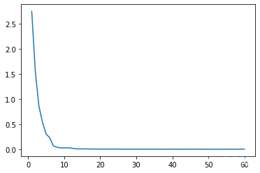
以下损失图分别为original、proposed结构的ResNet50的损失图，其6个单位(由数据集的数量及自定义参数num_print决定)为一次epoch。

import matplotlib.pyplot as plt

x =[ i+1for i inrange(len(loss_list))]# plot函数作图
plt.plot(x, loss_list)# show函数展示出这个图，如果没有这行代码，则程序完成绘图，但看不到
plt.show()

original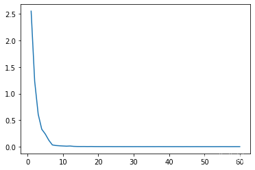

proposed

8. 模型验证

# 检验模式，不需要梯度更新
model.eval()
correct =0.0
total   =0with torch.no_grad():print("=======================check=======================")for inputs, labels in test_loader:# 从train_loader中取出batch_size个数据
        inputs, labels = inputs.to(device), labels.to(device)# 模型检验
        outputs = model(inputs)
        pred    = outputs.argmax(dim=1)#返回每一行中最大值的索引
        total   = total + inputs.size(0)
        correct = correct + torch.eq(pred, labels).sum().item()
            
        
    correct =100* correct/total
    print("Accuracy of the network on the 20094 test images:%.2f %%"%correct )print("===================================================")

9. 模型预测

数据集构建

"""
test为一个列表，存放图片的路径
其路径样式为asl_alphabet_test\\K_test.jpg
pre_test_dict为一个字典，如(种类:标号)
"""import torch
from PIL import Image
from torch.autograd import Variable
from torchvision import transforms
from torch.utils.data import Dataset, DataLoader

no_transform = transforms.Compose([
    transforms.Resize(224),
    transforms.ToTensor(),
    transforms.Normalize((0.51865010496974,0.49877608954906466,0.5143190141916275),(7.181780141103533,8.053991771959863,8.290017965464534))])# -----------------ready the dataset--------------------------defdefault_loader(path):
    img = Image.open(path)return img

classMyDataset(Dataset):# 构造函数def__init__(self, path, transform=None, target_transform=None, loader=default_loader):
        imgs =[]for img_path in path:
            temp      = img_path.split("\\")
            label     = temp[4][:-9]
            img_label = pre_test_dict[label]
            imgs.append((img_path,int(img_label),label))#imgs中包含有图像路径和标签
        self.path             = path
        self.imgs             = imgs
        self.transform        = transform
        self.target_transform = target_transform
        self.loader           = loader
        
    # hash_map建立def__getitem__(self, index):
        img_path, img_label, label = self.imgs[index]# 调用 opencv 打开图片
        img = self.loader(img_path)if self.transform isnotNone:
            img = self.transform(img)
        img_label -=1return img, img_path, label
    
    def__len__(self):returnlen(self.imgs)

test_data         = MyDataset(test, transform=no_transform)#test_data测试数据，调用DataLoader批量加载
test_loader         = DataLoader(dataset=test_data, batch_size=batch_size, shuffle=False)

模型预测

"""
test_dict为一个字典，如(标号:种类)
"""# 预测模式，不需要梯度更新
model.eval()with torch.no_grad():print("=======================forecast=======================")for inputs, img_paths, kind_labels in test_loader:# 从train_loader中取出batch_size个数据
        inputs = inputs.to(device)# 模型检验
        outputs      = model(inputs)
        pred         = outputs.argmax(dim=1).tolist()#返回每一行中最大值的索引for i inrange(len(pred)):
            predict = test_dict[pred[i]+1]
            path    = img_paths[i]
            real    = kind_labels[i]print("path: %s, predict: %s, real: %s"%(path, predict, real))print("===================================================")