
梯度下降 Gradient Descent
1.预备知识
1.1 什么是机器学习?
从翻译应用到自动驾驶汽车,机器学习 (ML) 技术为我们使用的一些最重要的技术提供支持。本课程介绍了机器学习背后的核心概念。
机器学习提供了一种解决问题和回答复杂问题的新方式。基本上,机器学习是指训练一个软件(称为模型)以从数据进行实用的预测的过程。机器学习模型表示机器学习系统用于进行预测的数据元素之间的数学关系。
例如,假设我们要创建一个预测降雨量的应用。我们可以使用传统方法或机器学习方法。我们使用传统的方法创建基于物理学的地球大气层和表面表征,计算大量的流体动力方程。这非常困难。
通过机器学习方法,我们将为机器学习模型提供大量天气数据,直到机器学习模型最终学习产生不同降水量的天气模式之间的数学关系。然后,我们会为模型提供当前天气数据,并预测降雨量。
机器学习系统类型
机器学习系统根据其学习进行预测的方式分为三类:
- 监督式学习
- 非监督式学习
- 强化学习
监督式学习
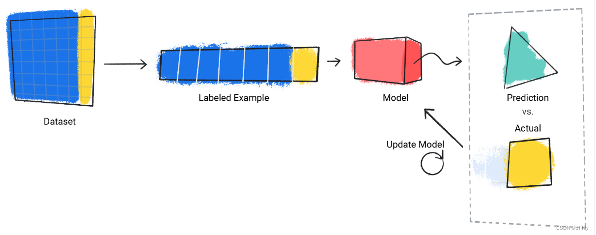
数据集由包含特征和标签的各个示例组成。您可以将示例视为电子表格中的单行。特征是受监管模型用于预测标签的值。标签是我们希望模型预测的“答案”或值。在用于预测降雨的天气模型中,特征可以是纬度、经度、温度、湿度、云度、风向和大气压力。标签将为 雨量。监督式学习涉及以下几个核心概念:
- 数据
- 模型
- 训练
- 评估
- 推断
- 1.数据
数据是机器学习的推动力。数据的形式是存储在表中的字词和数字,或者是图片和音频文件中捕获的像素和波形的值。我们将相关数据存储在数据集中。
数据是机器学习的推动力。数据的形式是存储在表中的字词和数字,或者是图片和音频文件中捕获的像素和波形的值。我们将相关数据存储在数据集中。
同时包含特征和标签的示例称为有标签样本。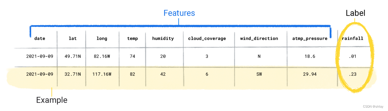
相比之下,无标签样本包含特征,但没有标签。创建模型后,模型会根据特征预测标签。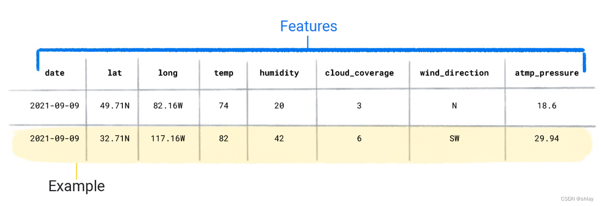
数据集的特征在于大小和多样性。大小是指样本的数量。多样性表示这些示例涵盖的范围。好的数据集既庞大又多样化。
- 2.模型
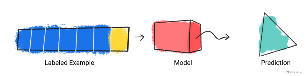
在监督式学习中,模型是一组复杂的数字,用于定义从特定输入特征模式到特定输出标签值的数学关系。模型会通过训练发现这些模式。
- 3.训练
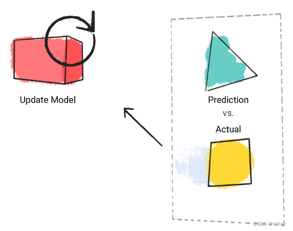
监督式学习模型必须先接受训练,然后才能进行预测。为了训练模型,我们会为模型提供一个包含有标签样本的数据集。该模型的目标是找出通过特征预测标签的最佳解决方案。该模型通过将其预测值与标签的实际值进行比较来确定最佳解决方案。根据预测值与实际值之间的差异(定义为损失),模型会逐步更新其解决方案。换言之,该模型会学习特征与标签之间的数学关系,以便对未见过的数据做出最佳预测。
例如,如果模型预测 1.15 inches 有雨,但实际值为 .75 inches,则模型会修改其解决方案,以使其预测更接近 .75 inches。模型查看数据集中的每个样本(在某些情况下多次)后,会得出平均为每个样本做出最佳预测的解决方案。
以下代码演示了如何训练模型:
- step1:该模型接受一个有标签样本,并提供预测。
- step2:模型将预测值与实际值进行比较,并更新其解决方案。
- step3:模型为数据集中的每个有标签样本重复此过程。
- 4.模型评估
我们会评估经过训练的模型,以确定它的学习效果。在评估模型时,我们使用的是带标签的数据集,但只会为模型提供数据集的特征。然后,我们会将模型的预测结果与标签的真实值进行比较。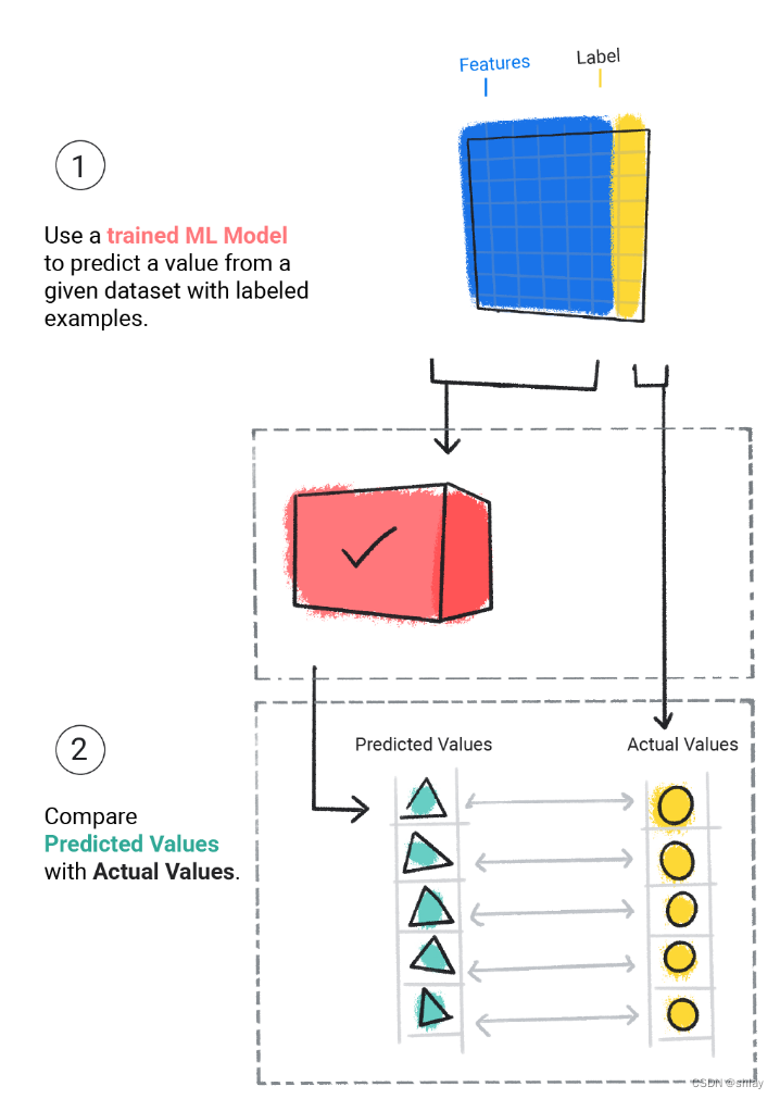
- 5.推断
在对评估模型的结果感到满意后,我们就可以使用该模型对无标签样本进行预测(称为推断)。在天气应用示例中,我们会为模型提供当前天气条件(例如温度、大气压力和相对湿度),同时还要预测降雨量。
1.2 几个专业术语
1.梯度下降(Gradient Descent)
:gradient
The vector of partial derivatives with respect to all of the independent variables. In machine learning, the gradient is the vector of partial derivatives of the model function. The gradient points in the direction of steepest ascent.
:gradient descent
A mathematical technique to minimize loss. Gradient descent iteratively adjusts weights and biases, gradually finding the best combination to minimize loss.
Gradient descent is older—much, much older—than machine learning.
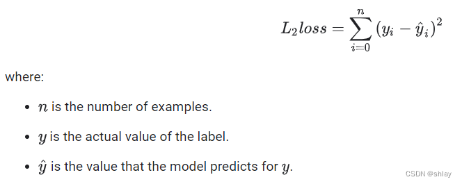
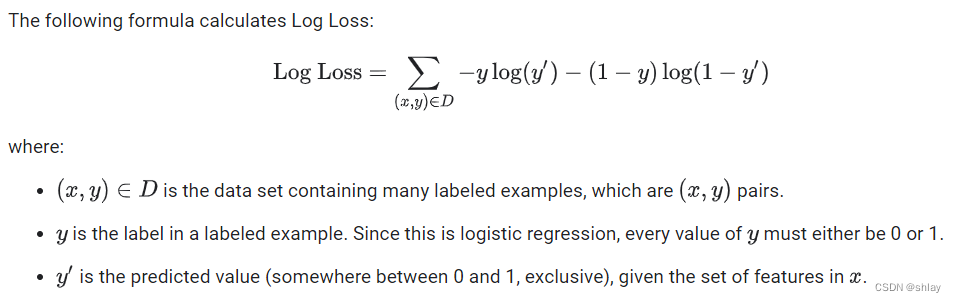
2.损失函数(loss function)
loss function
:
During training or testing, a mathematical function that calculates the loss on a batch of examples. A loss function returns a lower loss for models that makes good predictions than for models that make bad predictions.
The goal of training is typically to minimize the loss that a loss function returns.
Many different kinds of loss functions exist. Pick the appropriate loss function for the kind of model you are building. For example:
- 1.L2 loss (or Mean Squared Error) is the loss function for linear regression.
- 2.Log Loss is the loss function for logistic regression.
3.反向传播(Backpropagation)
backpropagation
:
The algorithm that implements gradient descent in neural networks.
Training a neural network involves many iterations of the following two-pass cycle:
During the forward pass, the system processes a batch of examples to yield prediction(s). The system compares each prediction to each label value. The difference between the prediction and the label value is the loss for that example. The system aggregates the losses for all the examples to compute the total loss for the current batch.
During the backward pass (backpropagation), the system reduces loss by adjusting the weights of all the neurons in all the hidden layer(s).
Neural networks often contain many neurons across many hidden layers. Each of those neurons contribute to the overall loss in different ways. Backpropagation determines whether to increase or decrease the weights applied to particular neurons.
The learning rate is a multiplier that controls the degree to which each backward pass increases or decreases each weight. A large learning rate will increase or decrease each weight more than a small learning rate.
In calculus terms, backpropagation implements calculus’ chain rule. That is, backpropagation calculates the partial derivative of the error with respect to each parameter. For more details, see this tutorial in Machine Learning Crash Course.
4.batch
- 1.
batch:
The set of examples used in one training iteration. The batch size determines the number of examples in a batch.
See epoch for an explanation of how a batch relates to an epoch.
- 2.
batch size:
The number of examples in a batch. For instance, if the batch size is 100, then the model processes 100 examples per iteration.
The following are popular batch size strategies:
Stochastic Gradient Descent (SGD), in which the batch size is 1.
full batch, in which the batch size is the number of examples in the entire training set. For instance, if the training set contains a million examples, then the batch size would be a million examples. Full batch is usually an inefficient strategy.
mini-batchin which the batch size is usually between 10 and 1000. Mini-batch is usually the most efficient strategy.
5.学习率(learning rate)
learning rate
:
A floating-point number that tells the gradient descent algorithm how strongly to adjust weights and biases on each iteration. For example, a learning rate of 0.3 would adjust weights and biases three times more powerfully than a learning rate of 0.1.
Learning rate is a key hyperparameter. If you set the learning rate too low, training will take too long. If you set the learning rate too high, gradient descent often has trouble reaching convergence.
During each iteration, the gradient descent algorithm multiplies the learning rate by the gradient. The resulting product is called the gradient step.
2. 前期准备
2.1 加载包
先下载我们的自写模块plots_lesson15.py
先下载我们的自写模块plots_lesson15.py
先下载我们的自写模块plots_lesson15.py
import numpy as np
from sklearn.linear_model import LinearRegression
from sklearn.preprocessing import StandardScaler
from plots_lesson15 import*%matplotlib inline
2.2 定义模型
       y


       =


       b


       +


       w


       x


       +


       ϵ


     \Large y = b + w x + \epsilon


 y=b+wx+ϵ
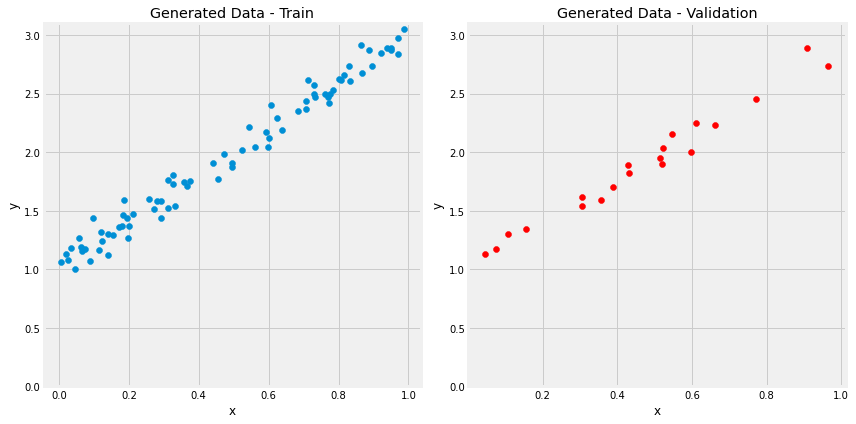
2.3 生成模拟数据
true_b =1
true_w =2
N =100# 生成数据
np.random.seed(42)
x = np.random.rand(N,1)
epsilon =(.1* np.random.randn(N,1))
y = true_b + true_w * x + epsilon
2.4 分割训练集验证集
# 打乱数据
idx = np.arange(N)
np.random.shuffle(idx)# 前80个样本作为训练集,剩余的作为验证集
train_idx = idx[:int(N*.8)]
val_idx = idx[int(N*.8):]

x_train, y_train = x[train_idx], y[train_idx]
x_val, y_val = x[val_idx], y[val_idx]
2.5 原始数据可视化
figure1(x_train, y_train, x_val, y_val)
3. 模型训练
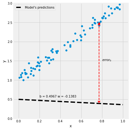
Step 0: 随机初始化待估参数
# Step 0 - 随机初始化参数 "b" 和 "w"
np.random.seed(42)
b = np.random.randn(1)
w = np.random.randn(1)print(b, w)
[0.49671415] [-0.1382643]
Step 1: 计算模型预测值
# Step 1 - 前向传播,根据参数计算模型的预测值
yhat = b + w * x_train
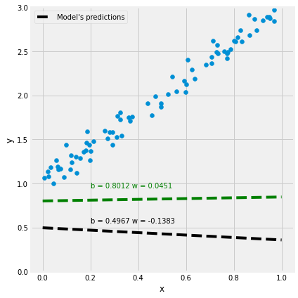
figure2(x_train, y_train, b, w)
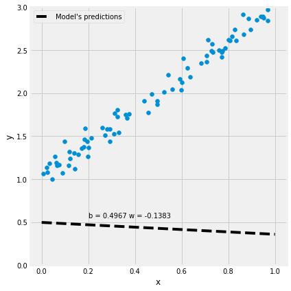
Step 2: 计算预测误差(模型损失)
error
i
=
y
i
^
−
y
i
\Large \text{error}_i = \hat{y_i} - y_i
errori=yi^−yi
figure3(x_train, y_train, b, w)
MSE
=
1
n
∑
i
=
1
n
error
i
2
=
1
n
∑
i
=
1
n
(
y
i
^
−
y
i
)
2
=
1
n
∑
i
=
1
n
(
b
+
w
x
i
−
y
i
)
2
\Large \begin{aligned} \text{MSE} &= \frac{1}{n} \sum_{i=1}^n{\text{error}_i}^2 \\ &= \frac{1}{n} \sum_{i=1}^n{(\hat{y_i} - y_i)}^2 \\ &= \frac{1}{n} \sum_{i=1}^n{(b + w x_i - y_i)}^2 \end{aligned}
MSE=n1i=1∑nerrori2=n1i=1∑n(yi^−yi)2=n1i=1∑n(b+wxi−yi)2
# Step 2 - 计算损失# 使用训练集中的所有样本计算损失值,这是BATCH gradient descent.

error =(yhat - y_train)# 损失函数用均方误差(mean squared error,MSE)
loss =(error **2).mean()print(loss)
2.7421577700550976
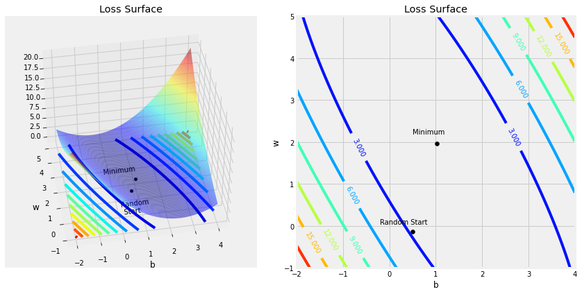
Step 2.1 计算损失面–Loss Surface
# 设定待估参数的值域范围,并将其进行100次等分割
b_range = np.linspace(true_b -3, true_b +3,101)
w_range = np.linspace(true_w -3, true_w +3,101)# 借助meshgrid 函数生成参数 b 和 w的取值网格
bs, ws = np.meshgrid(b_range, w_range)
bs.shape, ws.shape
((101, 101), (101, 101))
bs
array([[-2.  , -1.94, -1.88, ...,  3.88,  3.94,  4.  ],
       [-2.  , -1.94, -1.88, ...,  3.88,  3.94,  4.  ],
       [-2.  , -1.94, -1.88, ...,  3.88,  3.94,  4.  ],
       ...,
       [-2.  , -1.94, -1.88, ...,  3.88,  3.94,  4.  ],
       [-2.  , -1.94, -1.88, ...,  3.88,  3.94,  4.  ],
       [-2.  , -1.94, -1.88, ...,  3.88,  3.94,  4.  ]])
sample_x = x_train[0]
sample_yhat = bs + ws * sample_x
sample_yhat.shape
(101, 101)
all_predictions = np.apply_along_axis(
    func1d=lambda x: bs + ws * x,
    axis=1,
    arr=x_train
)
all_predictions.shape
(80, 101, 101)
all_labels = y_train.reshape(-1,1,1)
all_labels.shape
(80, 1, 1)
all_errors =(all_predictions - all_labels)
all_errors.shape
(80, 101, 101)
all_losses =(all_errors **2).mean(axis=0)
all_losses.shape
(101, 101)
figure4(x_train, y_train, b, w, bs, ws, all_losses)
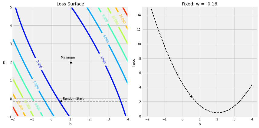
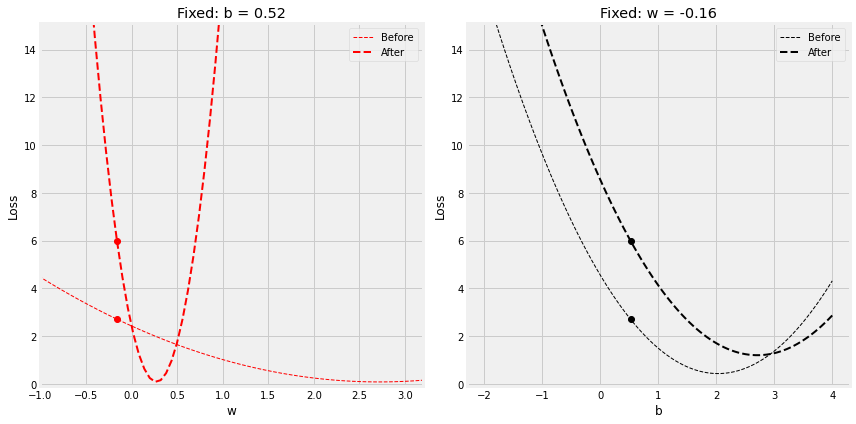
Step 2.2 损失横截面–Cross Sections
figure5(x_train, y_train, b, w, bs, ws, all_losses)
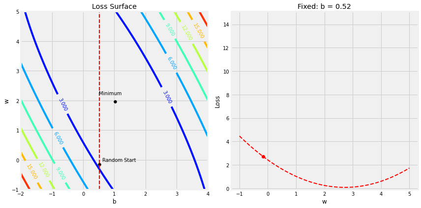
figure6(x_train, y_train, b, w, bs, ws, all_losses)
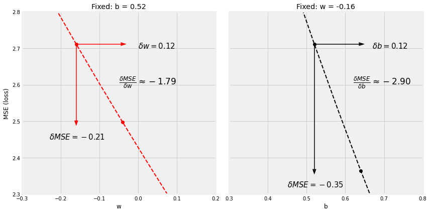
Step 3: 计算待估参数梯度- Gradients
∂
MSE
∂
b
=
∂
MSE
∂
y
i
^
∂
y
i
^
∂
b
=
1
n
∑
i
=
1
n
2
(
b
+
w
x
i
−
y
i
)
=
2
1
n
∑
i
=
1
n
(
y
i
^
−
y
i
)
∂
MSE
∂
w
=
∂
MSE
∂
y
i
^
∂
y
i
^
∂
w
=
1
n
∑
i
=
1
n
2
(
b
+
w
x
i
−
y
i
)
x
i
=
2
1
n
∑
i
=
1
n
x
i
(
y
i
^
−
y
i
)
\Large \begin{aligned} \frac{\partial{\text{MSE}}}{\partial{b}} = \frac{\partial{\text{MSE}}}{\partial{\hat{y_i}}} \frac{\partial{\hat{y_i}}}{\partial{b}} &= \frac{1}{n} \sum_{i=1}^n{2(b + w x_i - y_i)} \\ &= 2 \frac{1}{n} \sum_{i=1}^n{(\hat{y_i} - y_i)} \\ \frac{\partial{\text{MSE}}}{\partial{w}} = \frac{\partial{\text{MSE}}}{\partial{\hat{y_i}}} \frac{\partial{\hat{y_i}}}{\partial{w}} &= \frac{1}{n} \sum_{i=1}^n{2(b + w x_i - y_i) x_i} \\ &= 2 \frac{1}{n} \sum_{i=1}^n{x_i (\hat{y_i} - y_i)} \end{aligned}
∂b∂MSE=∂yi^∂MSE∂b∂yi^∂w∂MSE=∂yi^∂MSE∂w∂yi^=n1i=1∑n2(b+wxi−yi)=2n1i=1∑n(yi^−yi)=n1i=1∑n2(b+wxi−yi)xi=2n1i=1∑nxi(yi^−yi)
# Step 3 - 计算参数 "b" and "w" 的梯度
b_grad =2* error.mean()
w_grad =2*(x_train * error).mean()print(b_grad, w_grad)
-3.044811379650508 -1.8337537171510832
Step 3.1 梯度可视化
figure7(b, w, bs, ws, all_losses)
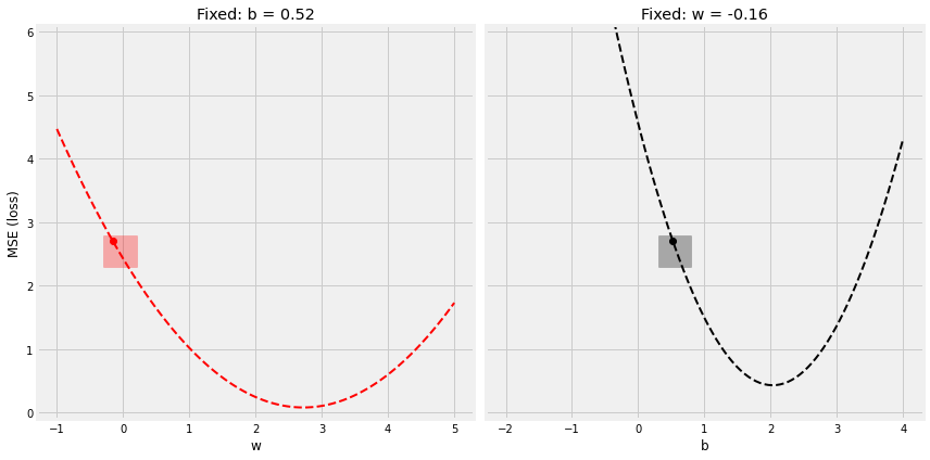
figure8(b, w, bs, ws, all_losses)
Step 3.2 反向传播–Backpropagation
Step 4: 更新待估参数
b
=
b
−
η
∂
MSE
∂
b
w
=
w
−
η
∂
MSE
∂
w
\Large \begin{aligned} b &= b - \eta \frac{\partial{\text{MSE}}}{\partial{b}} \\ w &= w - \eta \frac{\partial{\text{MSE}}}{\partial{w}} \end{aligned}
bw=b−η∂b∂MSE=w−η∂w∂MSE
# Sets 学习率(learning rate) - "eta"
lr =0.1print(b, w)# Step 4 - 利用梯度和学习率更新参数
b = b - lr * b_grad
w = w - lr * w_grad

print(b, w)
[0.49671415] [-0.1382643]
[0.80119529] [0.04511107]
利用更新后的参数b和w再次运行下面的step1至step4:
# Step 1 - 前向传播,根据参数计算模型的预测值
yhat = b + w * x_train

# Step 2 - 计算损失# 使用训练集中的所有样本计算损失值,这是BATCH gradient descent.
error =(yhat - y_train)# Step 3 - 计算参数 "b" and "w" 的梯度
b_grad =2* error.mean()
w_grad =2*(x_train * error).mean()print(b_grad, w_grad)# Step 4 - 利用梯度和学习率更新参数
b = b - lr * b_grad
w = w - lr * w_grad
print(b, w)
迭代多次可观察损失大小的变化以及估计值的变化
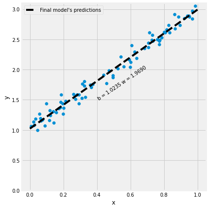
figure9(x_train, y_train, b, w)
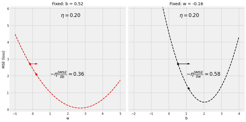
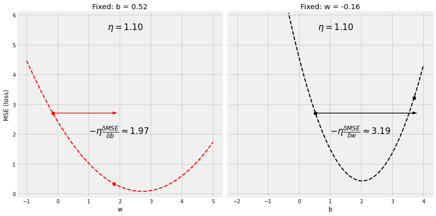
Step 4.1 学习率–Learning Rate
manual_grad_b =-2.90
manual_grad_w =-1.79

np.random.seed(42)
b_initial = np.random.randn(1)
w_initial = np.random.randn(1)
Step 4.1.1 低学习率
lr =0.2

figure10(b_initial, w_initial, bs, ws, all_losses, manual_grad_b, manual_grad_w, lr)
Step 4.1.2 高学习率
lr =0.8

figure10(b_initial, w_initial, bs, ws, all_losses, manual_grad_b, manual_grad_w, lr)

Step 4.1.3 非常高的学习率
lr =1.1
figure10(b_initial, w_initial, bs, ws, all_losses, manual_grad_b, manual_grad_w, lr)
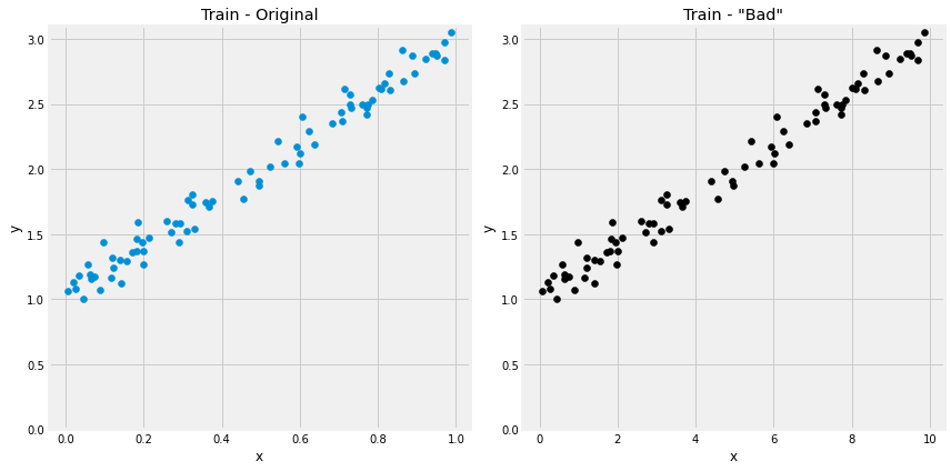
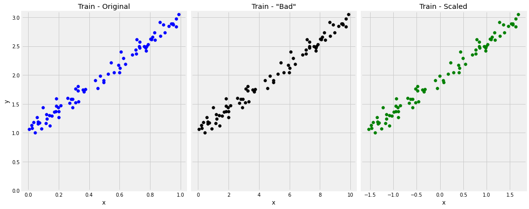
Step 4.2 坏的特征
true_b =1
true_w =2
N =100# 生成数据
np.random.seed(42)# w 除以 10
bad_w = true_w /10# x 乘以 10
bad_x = np.random.rand(N,1)*10# y保持不变
y = true_b + bad_w * bad_x +(.1* np.random.randn(N,1))
# 用同样的方式得到训练集和验证集数据
bad_x_train, y_train = bad_x[train_idx], y[train_idx]
bad_x_val, y_val = bad_x[val_idx], y[val_idx]
#对比初始的训练集和x,w进行变化后的训练集
fig, ax = plt.subplots(1,2, figsize=(12,6))
ax[0].scatter(x_train, y_train)
ax[0].set_xlabel('x')
ax[0].set_ylabel('y')
ax[0].set_ylim([0,3.1])
ax[0].set_title('Train - Original')
ax[1].scatter(bad_x_train, y_train, c='k')
ax[1].set_xlabel('x')
ax[1].set_ylabel('y')
ax[1].set_ylim([0,3.1])
ax[1].set_title('Train - "Bad"')
fig.tight_layout()
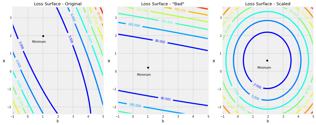
# w值域发声了改变所以我们需要重新得到参数b和w的取值网格
bad_b_range = np.linspace(-2,4,101)
bad_w_range = np.linspace(-2.8,3.2,101)
bad_bs, bad_ws = np.meshgrid(bad_b_range, bad_w_range)
figure14(x_train, y_train, b_initial, w_initial, bad_bs, bad_ws, bad_x_train)
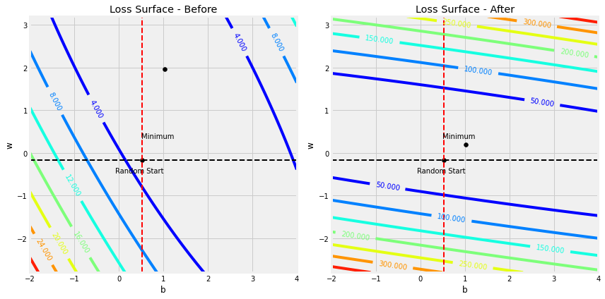
figure15(x_train, y_train, b_initial, w_initial, bad_bs, bad_ws, bad_x_train)
Step 4.3 特征标准化
X
‾
=
1
N
∑
i
=
1
N
x
i
σ
(
X
)
=
1
N
∑
i
=
1
N
(
x
i
−
X
‾
)
2
scaled
x
i
=
x
i
−
X
‾
σ
(
X
)
\Large \overline{X} = \frac{1}{N}\sum_{i=1}^N{x_i} \\ \Large \sigma(X) = \sqrt{\frac{1}{N}\sum_{i=1}^N{(x_i - \overline{X})^2}} \\ \Large \text{scaled } x_i=\frac{x_i-\overline{X}}{\sigma(X)}
X=N1i=1∑Nxiσ(X)=N1i=1∑N(xi−X)2scaled xi=σ(X)xi−X
scaler = StandardScaler(with_mean=True, with_std=True)# 只对训练集中的x进行标准化
scaler.fit(x_train)# 通过TRANSFORM函数标准化训练集和验证集中的特征x
scaled_x_train = scaler.transform(x_train)
scaled_x_val = scaler.transform(x_val)
#对比初始的训练集、x,w进行变化后坏的训练集、坏数据集的x标准化后的训练集
fig, ax = plt.subplots(1,3, figsize=(15,6))
ax[0].scatter(x_train, y_train, c='b')
ax[0].set_xlabel('x')
ax[0].set_ylabel('y')
ax[0].set_ylim([0,3.1])
ax[0].set_title('Train - Original')
ax[1].scatter(bad_x_train, y_train, c='k')
ax[1].set_xlabel('x')
ax[1].set_ylabel('y')
ax[1].set_ylim([0,3.1])
ax[1].set_title('Train - "Bad"')
ax[1].label_outer()
ax[2].scatter(scaled_x_train, y_train, c='g')
ax[2].set_xlabel('x')
ax[2].set_ylabel('y')
ax[2].set_ylim([0,3.1])
ax[2].set_title('Train - Scaled')
ax[2].label_outer()

fig.tight_layout()
# 再次重新设定w和b的取值网格
scaled_b_range = np.linspace(-1,5,101)
scaled_w_range = np.linspace(-2.4,3.6,101)
scaled_bs, scaled_ws = np.meshgrid(scaled_b_range, scaled_w_range)
figure17(x_train, y_train, scaled_bs, scaled_ws, bad_x_train, scaled_x_train)
Step 5: 反复更新参数
figure18(x_train, y_train)
版权归原作者 shlay 所有, 如有侵权,请联系我们删除。