基于时空序列模型ConvLstm的气象预测

一、数据获取

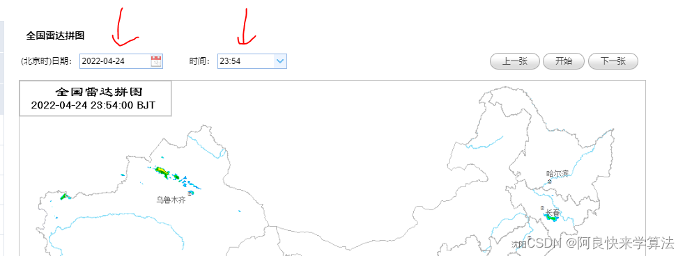
1. 去国家气象科学数据中心下载雷达拼图 可以手动收集也可以写爬虫程序收集 手动收集就更改日期和时间中国气象数据网 - Online Data

二、数据预处理

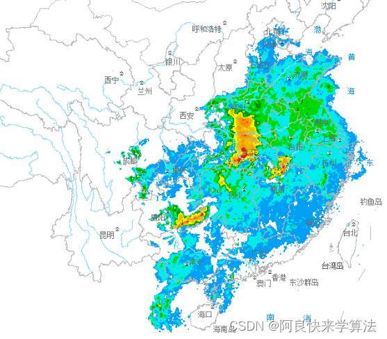
1. 得到这些PNG图片后，首先做处理，只关注东南部分，其他的都扔掉（即从图中截取一个固定的长方形，就差不多是下面这个部分。保证截取的图中不包括左下角的南海诸岛以及右下角的基本反射率图例，这些都是干扰。你可以扔掉更多的部分，比如西宁以西都扔掉）。对所有的PNG图片都这样操作。

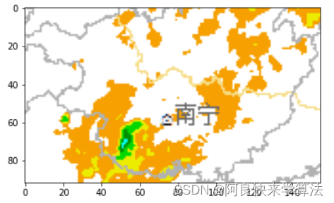
2. 可能截取完之后，图片的像素仍然过多，那你可以截取更小的一个部分。比如：pic_name_listcuted_img_list = []save_img_path = os.path.join(wd, 'output')if not os.path.exists(save_img_path): os.makedirs(save_img_path) for pic_id in range(len(pic_name_list)): pic_name = str(pic_id) + '.png' temp = os.path.join(pic_root_path, pic_name) img = cv.imread(temp) print("This is the "+pic_name+":") print(img.shape) # (y, x) cuted_img = img[633:725, 510:665] #cv.imwrite(os.path.join(save_img_path, pic_name),cuted_img) cuted_img_list.append(cuted_img) plt.imshow(cuted_img) plt.show()

3. 识别出基本反射率图例中每一个不同数值对应的颜色RGB常数，将图片中每个像素的RGB映射到基本反射率。如果没有对应的值（比如白色，黑色）统统设置为255。

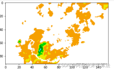
4. 转为灰度图。

    ![](https://img-blog.csdnimg.cn/c6b726f5c6194da9a5b35e34b1ccbad7.png)
   

def viewColor(pic, color):
    #pic = Image.copy()
    for i, nar in enumerate(pic):
        for j, n in enumerate(nar):
            if list(n) == list(color): # 南宁附近的三八线不需要的
                pic[i][j] = np.array([255,255,255])
    
def get_usedColor(img):
    from collections import defaultdict
    colorMap = defaultdict(int)
    usedColor = []
    
    for i, nar in enumerate(img):
        for j, n in enumerate(nar):
            if str(n) not in colorMap:
                usedColor.append(list(n))
            colorMap[str(n)] += 1
    return usedColor
    
def Image_Preprocessing(img):
    use_color = []
    use_color.append([178, 178, 178])
    use_color.append([247, 221, 136])
    use_color.append([104, 104, 104])
    use_color.append([182, 255, 255])
    use_color.append([0, 0, 102])
    use_color.append([219, 144, 58])
    use_color.append([58, 144, 219])
    use_color.append([102, 0, 0])
    use_color.append([255, 255, 182])
    use_color.append([219, 255, 255])
    use_color.append([219, 182, 182])
    use_color.append([219, 144, 144])
    use_color.append([219, 219, 219])
    use_color.append([0, 58, 144])
    use_color.append([182, 182, 182])
    use_color.append([0, 0, 0])
    use_color.append([58, 0, 0])
    use_color.append([255, 219, 144])
    for c in use_color:
        viewColor(img, c)
    return img

def pltShow(img):
    plt.imshow(img)
    plt.show()
    
def cvShow(img):
    cv.imshow("mat", img)
    cv.waitKey(0)

imgGray_list = []
for id, cuted_img in enumerate(cuted_img_list):
    img = Image_Preprocessing(cuted_img)
    imgGray = cv.cvtColor(img, cv.COLOR_BGR2GRAY)
    pltShow(img)
    temp = os.path.join(save_img_path, str(id)+'.png')
    if os.path.exists(temp):
        os.remove(temp)
    cv.imwrite(temp, imgGray)
    imgGray_list.append(imgGray)
    print(str(id)+'.png is preprocesed, Wait next!')
print("Everything is OK!")

三、ConvLstm模型

## NEW NETWORK ##
def mainmodel():
  # Inputs
  dtype='float32'

  nk = 128     # number of kernels for conv layers #48 
  fs = (3,3)  # filter size for convolutional kernels
  
  contentInput = Input(shape=(None, WIDTH, HEIGHT, 1), name='content_input', dtype=dtype)

  # Encoding Network
  x1 = ConvLSTM2D(nk, (5,5), padding='same', return_sequences=True, kernel_initializer ='he_normal', name='layer1')(contentInput)
  x2 = ConvLSTM2D(nk, (5,5), padding='same', return_sequences=True, kernel_initializer ='he_normal', name='layer2')(x1) 

  # Forecasting Network
  x3 = ConvLSTM2D(nk, (5,5), padding='same', return_sequences=True, kernel_initializer ='he_normal', name='layer3')(x1)
  add1 = Add()([x3, x2])
  x4 = ConvLSTM2D(nk, (5,5), padding='same', return_sequences=True, kernel_initializer ='he_normal', name='layer4')(add1)

  # Prediction Network
  conc = Concatenate()([x4, x3]) 
  predictions = Conv3D(1, (5,5,5), activation='sigmoid', padding='same',  name='prediction')(conc) #sigmoid original

  model = Model(inputs=contentInput, outputs=predictions)
  
  return model

四、训练

## NEW NETWORK ##
def mainmodel():
  # Inputs
  dtype='float32' 

  nk = 128     # number of kernels for conv layers #48 
  fs = (3,3)  # filter size for convolutional kernels
  
  contentInput = Input(shape=(None, WIDTH, HEIGHT, 1), name='content_input', dtype=dtype)

  # Encoding Network
  x1 = ConvLSTM2D(nk, (5,5), padding='same', return_sequences=True, kernel_initializer ='he_normal', name='layer1')(contentInput)
  x2 = ConvLSTM2D(nk, (5,5), padding='same', return_sequences=True, kernel_initializer ='he_normal', name='layer2')(x1) 

  # Forecasting Network
  x3 = ConvLSTM2D(nk, (5,5), padding='same', return_sequences=True, kernel_initializer ='he_normal', name='layer3')(x1)
  add1 = Add()([x3, x2])
  x4 = ConvLSTM2D(nk, (5,5), padding='same', return_sequences=True, kernel_initializer ='he_normal', name='layer4')(add1)

  # Prediction Network
  conc = Concatenate()([x4, x3]) 
  predictions = Conv3D(1, (5,5,5), activation='sigmoid', padding='same',  name='prediction')(conc) #sigmoid original

  model = Model(inputs=contentInput, outputs=predictions)
  
  return model

# Train model
def train(main_model=True, batchsize=5, epochs=50, save=False):

  smooth=1e-9
  #Additional metrics: SSIM, PSNR, POD, FAR
  def ssim(x, y, max_val=1.0):
    return tf.image.ssim(x, y, max_val)

  def psnr(x, y, max_val=1.0):
    return tf.image.psnr(x, y, max_val)

  #recall
  def POD(x, y):
    y_pos = K.clip(x, 0, 1)
    y_pred_pos = K.clip(y, 0, 1)
    y_pred_neg = 1 - y_pred_pos
    tp = K.sum(y_pos * y_pred_pos)
    fn = K.sum(y_pos * y_pred_neg)
    return (tp+smooth)/(tp+fn+smooth)

  def FAR(x, y):
    y_pred_pos = K.clip(y, 0, 1)
    y_pos = K.clip(x, 0, 1)
    y_neg = 1 - y_pos
    tp = K.sum(y_pos * y_pred_pos)
    fp = K.sum(y_neg * y_pred_pos)
    return (fp)/(tp+fp+smooth)

  metrics = ['accuracy', ssim, psnr, POD, FAR]

  global history, model

  if main_model:
    model=mainmodel()
    print("[INFO] Compiling Main Model...")
    optim = Adam(lr=0.001, beta_1=0.9, beta_2=0.999, amsgrad=False)
    model.compile(loss='logcosh', optimizer=optim, metrics=metrics) #logcosh gives better results than crossentropy or mse 
    print("[INFO] Compiling Main Model: DONE")
    print("[INFO] Training Main Model...")
    history = model.fit(INPUT_SEQUENCE[:40], NEXT_SEQUENCE[:40], batch_size=batchsize, epochs=epochs, validation_split=0.1, verbose=1, use_multiprocessing=True)
    print("[INFO] Training of Main Model: DONE")
    #Save trained model  
    if save:
      print("[INFO] Saving Model...")
      #model.save('models/model1_ConvLSTM/mainmodel_1.h5')
      # serialize model to JSON
      model_json = model.to_json()
      with open("models/model1_ConvLSTM/mainmodel_1.json", "w") as json_file:
          json_file.write(model_json)
      # serialize weights to HDF5
      model.save_weights("models/model1_ConvLSTM/mainmodel_1.h5")
      print("[INFO] Model Saved")
    else: print("[INFO] Model not saved")
  else:
    model=test_model()
    print("[INFO] Compiling Test Model...")
    model.compile(loss='logcosh', optimizer='adam', metrics=metrics)
    print("[INFO] Compiling Test Model: DONE")
    print("[INFO] Training Test Model...:")
    #history = model.fit(INPUT_SEQUENCE[:40], NEXT_SEQUENCE[:40], batch_size=5, epochs=180, validation_split=0.05, verbose=1, use_multiprocessing=True)
    history = model.fit(INPUT_SEQUENCE[:60], NEXT_SEQUENCE[:60], batch_size=batchsize, epochs=epochs, validation_split=0.05, verbose=1, use_multiprocessing=True)
    print("[INFO] Training of Test Model: DONE")
    #Save trained model 
    if save:
      print("[INFO] Saving Test Model...")
      model.save('models/model1_ConvLSTM/trained_test_model_samples.h5')
      print("[INFO] Model Saved")
    else: print("[INFO] Model not saved")

### PLOT LOSS vs EPOCHS ###

def performance(): 
  # Plot training & validation accuracy values
  plt.plot(history.history['acc'])
  plt.plot(history.history['val_acc'])
  plt.title('Model accuracy')
  plt.ylabel('Accuracy')
  plt.xlabel('Epoch')
  plt.legend(['Train', 'Test'], loc='upper left')
  plt.show()
  # Plot training & validation loss values
  plt.plot(history.history['loss'])
  plt.plot(history.history['val_loss'])
  plt.title('Model loss')
  plt.ylabel('Loss')
  plt.xlabel('Epoch')
  plt.legend(['Train', 'Test'], loc='upper left')
  plt.show()
  # Plot POD/FAR plot
  plt.plot(history.history['POD'])
  plt.plot(history.history['FAR'])
  plt.title('POD, FAR plot')
  plt.ylabel('POD / FAR')
  plt.xlabel('Epoch')
  plt.legend(['POD', 'FAR'], loc='upper left')
  plt.show()

#Train Model

#main_model = True  trains main_model
#main_model = False trains test_model

train(main_model=True, batchsize=4, epochs=8, save=True)

五、预测

（待补）