基于GMM的一维时序数据平滑算法

本文将介绍我们使用高斯混合模型(GMM)算法作为一维数据的平滑和去噪算法。

假设我们想要在音频记录中检测一个特定的人的声音，并获得每个声音片段的时间边界。例如，给定一小时的流，管道预测前10分钟是前景(我们感兴趣的人说话)，然后接下来的20分钟是背景(其他人或没有人说话)，然后接下来的20分钟是前景段，最后10分钟属于背景段。

有一种方法是预测每个语音段的边界，然后对语音段进行分类。但是如果我们错过了一个片段，那么这个错误将会使整个片段产生错误。想要解决这题我们可以使用GMM smooth，音频检测器生成时间范围片段和每个片段的标签。GMM smooth的输入数据是这些段，它可以帮助我们来降低最终预测中的噪声。

高斯混合模型

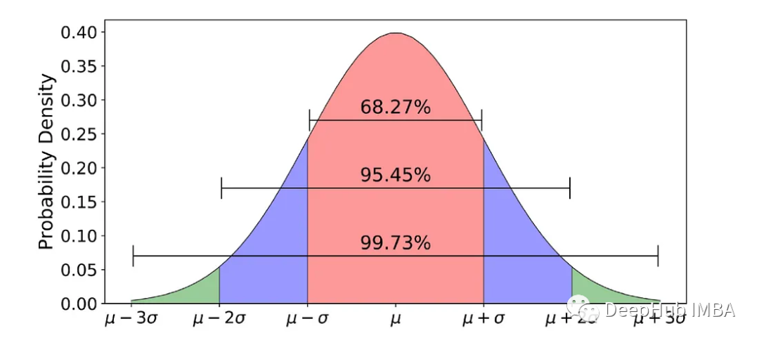
在深入GMM之前，必须首先了解高斯分布。高斯分布是一种概率分布，由两个参数定义:平均值(或期望)和标准差(STD)。在统计学中，平均值是指数据集的平均值，而标准偏差(STD)衡量数据的变化或分散程度。STD表示每个数据点与平均值之间的距离，在高斯分布中，大约68%的数据落在平均值的一个STD内。

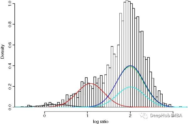
GMM是一种参数概率模型。它假设在给定的一组数据点中，每一个单点都是由一个高斯分布产生的，给定一组K个高斯分布[7]。GMM的目标是从K个分布中为每个数据点分配一个高斯分布。换句话说，GMM解决的任务是聚类任务或无监督任务。

GMMs通常用作生物识别系统中连续测量或特征的概率分布的参数模型，例如说话人识别系统中与声道相关的频谱特征。使用迭代期望最大化(EM)算法或来自训练良好的先验模型的最大后验(MAP)估计从训练数据中估计GMM参数[8]。

基于 GMM 的平滑器

我们的目标是解决时间概念定位问题，比如输出如下所示：[[StartTime1, EndTime1, Class1], [StartTime2, EndTime2, Class2], …]。如果我们想直观地展示一下，可以像下图这样：

但是因为误差而产生很大的噪声，如下所示:

我们的目标只是减少噪声(并使用本文后面描述的方法测量噪声)。可以看到背景预测更常见（橙色），也就是说我们正在寻找的说话者的“标记”音频片段更频繁地被预测为“其他说话者”或“没有说话”。

可以看到噪声预测与真实预测相比具有较小的长度，所以可以得出结论，噪声预测是可以与真实预测分离的。我们将预测的长度建模为高斯分布的混合，使用GMM作为噪声平滑算法来解决这个问题。

代码和解释

完整的代码可以在下面的代码块中看到:

 fromcopyimportdeepcopy
 importnumpyasnp
 frommatplotlibimportpyplotasplt
 importpandasaspd
 fromsklearn.mixtureimportGaussianMixture
 importlogging
 logger=logging.getLogger()
 logger.setLevel(logging.INFO)
 logger.addHandler(logging.StreamHandler())
 
 classGMMSmoother:
     """
     This class is the main class of the Smoother. It performs a smoothing to joint segments
     """
     def__init__(self, min_samples=10):
         # The minimum number of samples for applying GMM
         self.min_samples=min_samples
         # Logger instance
         self.logger=logger
     defsmooth_segments_gmm(self, segments, gmm_segment_class='background', bg_segment_class='foreground'):
         """
         This method performs the smoothing using Gaussian Mixture Model (GMM) (for more information about GMM
         please visit: https://scikit-learn.org/stable/modules/mixture.html). It calculates two GMMs: first with one
         gaussian component and the second with two components. Then, it selects the best model using AIC, and BIC metrics.
         After we choose the best model, we perform a clustering of tew clusters: real or fake
         Please note that the GMMs don't use the first and last segments because in our case
         the stream's time limit is an hour and we don't have complete statistics on 
         the lengths of the first and last segments.
         :param segments: a list of dictionaries, each dict represents a segment
         :param gmm_segment_class: the segment class of the "reals"
         :param bg_segment_class: the segment class of the "fakes"
         :return:
         segments_copy: the smoothed version of segments
         """
         self.logger.info("Begin smoothing using Gaussian Mixture Model (GMM)")
         # Some instancing 
         preds_map= {0: bg_segment_class, 1: gmm_segment_class}
         gmms_results_dict= {}
         # Copy segments to a new variable
         segments_copy=deepcopy(segments)
         self.logger.info("Create input data for GMM")
         # Keep the gmm_segment_class data points and perform GMM on them.
         # For example: gmm_segment_class = 'background'
         segments_filtered= {i: sfori, sinenumerate(segments_copy) if
                           s['segment'] ==gmm_segment_classand (i>0andi<len(segments_copy) -1)}
         # Calcualte the length of each segment
         X=np.array([[(s['endTime'] -s['startTime']).total_seconds()] for_, sinsegments_filtered.items()])
         # Check if the length of data points is less than the minimum. 
         # If it is, do not apply GMM!
         iflen(X) <=self.min_samples:
             self.logger.warning(f"Size of input ({len(X)} smaller than min simples ({self.min_samples}). Do not perform smoothing.)")
             returnsegments
         # Go over 1 and 2 components and calculate statistics
         best_fitting_score=np.Inf
         self.logger.info("Begin to fit GMMs with 1 and 2 components.")
         foriin [1, 2]: 
             # For each number of component (1 or 2), fit GMM
             gmm=GaussianMixture(n_components=i, random_state=0, tol=10**-6).fit(X)
             # Calculate AIC and BIC and the average between them
             aic, bic=gmm.aic(X), gmm.bic(X)
             fitting_score= (aic+bic) /2
             # If the average is less than the best score, replace them
             iffitting_score<best_fitting_score:
                 best_model=gmm
                 best_fitting_score=fitting_score
             gmms_results_dict[i] = {"model": gmm, "fitting_score": fitting_score, "aic": aic, "bic": bic}
         self.logger.info(f"GMM with {best_model.n_components} components was selected")
         # If the number of components is 1, change the label to the points that
         # have distance from the mean that is bigger than 2*STD
         ifbest_model.n_components==1:
             mean=best_model.means_[0, 0]
             std=np.sqrt(best_model.covariances_[0, 0])
             model_preds= [0ifx<mean-2*stdelse1forxinrange(len(X))]
         # If the number of components is 2, assign a label to each data point,
         # and replace the label to the points that assigned to the low mean Gaussian
         else:
             ifnp.linalg.norm(best_model.means_[0]) >np.linalg.norm(best_model.means_[1]):
                 preds_map= {1: bg_segment_class, 0: gmm_segment_class}
             model_preds=best_model.predict(X)
         self.logger.info("Replace previous predictions with GMM predictions")
         # Perform smoothing
         fori, (k, s) inenumerate(segments_filtered.items()):
             ifs['segment'] !=preds_map[model_preds[i]]:
                 s['segment'] =preds_map[model_preds[i]]
                 segments_copy[k] =s
         self.logger.info("Merge segments")
         # Join consecutive segments after the processing
         segments_copy=join_consecutive_segments(segments_copy)
         returnsegments_copy
     @staticmethod
     defplot_bars(res_dict_objs, color_dict={"foreground": "#DADDFC", "background": '#FC997C', "null": "#808080"}, channel="",
                   start_time="", end_time="", snrs=None, titles=['orig', 'smoothed'],
                   save=False, save_path="", show=True):
         """
         Inspired by https://stackoverflow.com/questions/70142098/stacked-horizontal-bar-showing-datetime-areas
         This function is for visualizing the smoothing results 
         of multiple segments' lists
         :param res_dict_objs: a list of lists. Each list is a segments list to plot
         :param color_dict: dictionary which represents the mapping between class to color in the plot
         :param channel: channel number
         :param start_time: absolute start time
         :param end_time: absolute end time
         :param snrs: list of snrs to display in the title
         :param titles: title to each subplot
         :param save: flag to save the figure into a png file
         :param save_path: save path of the figure
         :param show: flag to show the figure
         """
         ifsnrs==None:
             snrs= [''] *len(res_dict_objs)
         iftype(res_dict_objs) !=list:
             res_dict_objs= [res_dict_objs]
         fig, ax=plt.subplots(len(res_dict_objs), 1, figsize=(20, 10))
         fig.suptitle(f"Channel {channel}, {start_time}-{end_time}\n{snrs[0]}\n{snrs[1]}")
         fordict_idx, res_dictinenumerate(res_dict_objs):
             date_from= [a['startTime'] forainres_dict]
             date_to= [a['endTime'] forainres_dict]
             segment= [a['segment'] forainres_dict]
             df=pd.DataFrame({'date_from': date_from, 'date_to': date_to,
                                'segment': segment})
             foriinrange(df.shape[0]):
                 ax[dict_idx].plot([df['date_from'][i], df['date_to'][i]], [1, 1],
                                   linewidth=50, c=color_dict[df['segment'][i]])
             ax[dict_idx].set_yticks([])
             ax[dict_idx].set_yticklabels([])
             ax[dict_idx].set(frame_on=False)
             ax[dict_idx].title.set_text(titles[dict_idx])
         ifshow:
             plt.show()
         ifsave:
             plt.savefig(save_path)
 defjoin_consecutive_segments(seg_list):
     """
     This function is merged consecutive segments if they 
     have the same segment class and create one segment. It also changes the
     start and the end times with respect to the joined segments
     :param seg_list: a list of dictionaries. Each dict represents a segment
     :return: joined_segments: a list of dictionaries, where the segments are merged
     """
     joined_segments=list()
     init_seg= {
         'startTime': seg_list[0]['startTime'],
         'endTime': seg_list[0]['endTime'],
         'segment': seg_list[0]['segment']
     }
     collector=init_seg
     last_segment=init_seg
     last_segment=last_segment['segment']
     forseginseg_list:
         segment=seg['segment']
         start_dt=seg['startTime']
         end_dt=seg['endTime']
         prefiltered_type=segment
         ifprefiltered_type==last_segment:
             collector['endTime'] =end_dt
         else:
             joined_segments.append(collector)
             init_seg= {
                 'startTime': start_dt,
                 'endTime': end_dt,
                 'segment': prefiltered_type
             }
             collector=init_seg
             last_segment=init_seg
             last_segment=last_segment['segment']
     joined_segments.append(collector)
     returnjoined_segments
 defmain(seg_list):
     # Create GMMSmoother instance
     gmm_smoother=GMMSmoother()
     # Join consecutive segments that have the same segment label
     seg_list_joined=join_consecutive_segments(seg_list)
     # Perform smoothing on background class
     smoothed_segs_tmp=gmm_smoother.smooth_segments_gmm(seg_list_joined)
     # Perform smoothing on foreground class
     smoothed_segs_final=gmm_smoother.smooth_segments_gmm(smoothed_segs_tmp, gmm_segment_class='foreground', bg_segment_class='background') iflen(
         smoothed_segs_tmp) !=len(seg_list_joined) elsesmoothed_segs_tmp
     returnsmoothed_segs_final
 if__name__=="__main__":
     # The read_data_func should be implemented by the user,
     # depending on his needs.
     seg_list=read_data_func()
     res=main(seg_list)

下面我们解释关键块以及如何使用GMM来执行平滑:

1、输入数据

数据结构是一个字典列表。每个字典代表一个段预测，具有以下键值对: “startTime”，“endTime”和“segment”。下面是一个例子:

 {"startTime": ISODate("%Y-%m-%dT%H:%M:%S%z"), "endTime": ISODate("%Y-%m-%dT%H:%M:%S%z"), "segment": "background/foreground"}

“startTime”和“endTime”是段的时间边界，“segment”是它的类型。

2、连接连续段

假设输入数据具有相同标签的连续预测(并非所有输入数据都必须需要此阶段)。例如:

 # Input segments list
 seg_list = [{"startTime": ISODate("2022-11-19T00:00:00Z"), "endTime": ISODate("2022-11-19T01:00:00Z"), "segment": "background"}, 
 {"startTime": ISODate("2022-11-19T01:00:00Z"), "endTime": ISODate("2022-11-19T02:00:00Z"), "segment": "background"}]
 # Apply join_consecutive_segments on seg_list to join consecutive segments
 seg_list_joined = join_consecutive_segments(seg_list)
 # After applying the function, the new list should look like the following:
 # seg_list_joined = [{"startTime": ISODate("2022-11-19T00:00:00Z"), "endTime": ISODate("2022-11-19T02:00:00Z"), "segment": "background"}]

使用的join_consecutive_segments的代码如下:

 defjoin_consecutive_segments(seg_list):
     """
     This function is merged consecutive segments if they 
     have the same segment class and create one segment. It also changes the
     start and the end times with respect to the joined segments
     :param seg_list: a list of dictionaries. Each dict represents a segment
     :return: joined_segments: a list of dictionaries, where the segments are merged
     """
     joined_segments=list()
 
     init_seg= {
             'startTime': seg_list[0]['startTime'],
             'endTime': seg_list[0]['endTime'],
             'segment': seg_list[0]['segment']
         }
         collector=init_seg
         last_segment=init_seg
         last_segment=last_segment['segment']
         forseginseg_list:
             segment=seg['segment']
             start_dt=seg['startTime']
             end_dt=seg['endTime']
             prefiltered_type=segment
             ifprefiltered_type==last_segment:
                 collector['endTime'] =end_dt
             else:
                 joined_segments.append(collector)
                 init_seg= {
                     'startTime': start_dt,
                     'endTime': end_dt,
                     'segment': prefiltered_type
                 }
                 collector=init_seg
                 last_segment=init_seg
                 last_segment=last_segment['segment']
         joined_segments.append(collector)
         returnjoined_segments

join_consecutive_segments将两个或多个具有相同预测的连续片段连接为一个片段。

3、删除当前迭代的不相关片段

我们的预测有更多的噪声，所以首先需要对它们进行平滑处理。从数据中过滤掉前景部分：

 # Copy segments to a new variable
 segments_copy=deepcopy(segments)
 # Keep the gmm_segment_class data points and perform GMM on them.
 # For example: gmm_segment_class = 'background'
 segments_filtered= {i: sfori, sinenumerate(segments_copy) ifs['segment'] ==gmm_segment_classand (i>0andi<len(segments_copy) -1)}

4、计算段的长度

以秒为单位计算所有段的长度。

 # Calcualte the length of each segment
 X=np.array([[(s['endTime'] -s['startTime']).total_seconds()] for_, sinsegments_filtered.items()])

5、GMM

仅获取背景片段的长度并将 GMM 应用于长度数据。如果有足够的数据点（预定义数量——超参数），我们这里使用两个GMM：一个分量模型和两个分量模型。然后使用贝叶斯信息准则 (BIC) 和 Akaike 信息准则 (AIC) 之间的平均值来选择最适合的 GMM。

 # Check if the length of data points is less than the minimum. 
 # If it is, do not apply GMM!
 iflen(X) <=self.min_samples:
     self.logger.warning(f"Size of input ({len(X)} smaller than min simples ({self.min_samples}). Do not perform smoothing.)")
     returnsegments
 # Go over 1 and 2 number of components and calculate statistics
 best_fitting_score=np.Inf
 self.logger.info("Begin to fit GMMs with 1 and 2 components.")
 foriinrange(1, 3): 
     # For each number of component (1 or 2), fit GMM
     gmm=GaussianMixture(n_components=i, random_state=0, tol=10**-6).fit(X)
     # Calculate AIC and BIC and the average between them
     aic, bic=gmm.aic(X), gmm.bic(X)
     fitting_score= (aic+bic) /2
     # If the average is less than the best score, replace them
     iffitting_score<best_fitting_score:
         best_model=gmm
         best_fitting_score=fitting_score
     gmms_results_dict[i] = {"model": gmm, "fitting_score": fitting_score, "aic": aic, "bic": bic}

6、选择最佳模型并进行平滑

如果选择了一个分量：将距离均值大于 2-STD 的数据点标记为前景，其余数据点保留为背景点。

如果选择了两个分量：将分配给低均值高斯的点标记为前景，将高均值高斯标记为背景。

 # If the number of components is 1, change the label to the points that
 # have distance from the mean that is bigger than 2*STD
 ifbest_model.n_components==1:
     mean=best_model.means_[0, 0]
     std=np.sqrt(best_model.covariances_[0, 0])
     model_preds= [0ifx<mean-2*stdelse1forxinrange(len(X))]
 # If the number of components is 2, assign a label to each data point,
 # and replace the label to the points that assigned to the low mean Gaussian
 else:
     ifnp.linalg.norm(best_model.means_[0]) >np.linalg.norm(best_model.means_[1]):
         preds_map= {1: bg_segment_class, 0: gmm_segment_class}
     model_preds=best_model.predict(X)
 self.logger.info("Replace previous predictions with GMM predictions")
 # Perform smoothing
 fori, (k, s) inenumerate(segments_filtered.items()):
     ifs['segment'] !=preds_map[model_preds[i]]:
         s['segment'] =preds_map[model_preds[i]]
         segments_copy[k] =s
 self.logger.info("Merge segments")

7、后处理

再次连接连续的片段产生并返回最终结果。

 # Join consecutive segments after the processing
 segments_copy=join_consecutive_segments(segments_copy)

8、重复这个过程

这是一个迭代的过程我们可以重复这个过程几次，来找到最佳结果

9、可视化

使用下面方法可以可视化我们的中间和最终的结果，并方便调试

 defplot_bars(res_dict_objs, color_dict={"foreground": "#DADDFC", "background": '#FC997C', "null": "#808080"}, channel="",
               start_time="", end_time="", snrs=None, titles=['orig', 'smoothed'],
               save=False, save_path="", show=True):
     """
     This function is for visualizing the smoothing results of multiple segments lists
     :param res_dict_objs: a list of lists. Each list is a segments list to plot
     :param color_dict: dictionary which represents the mapping between class to color in the plot
     :param channel: channel number
     :param start_time: absolute start time
     :param end_time: absolute end time
     :param snrs: list of snrs to display in the title
     :param titles: title to each subplot
     :param save: flag to save the figure into a png file
     :param save_path: save path of the figure
     :param show: flag to show the figure
     """
     ifsnrs==None:
         snrs= [''] *len(res_dict_objs)
     iftype(res_dict_objs) !=list:
         res_dict_objs= [res_dict_objs]
     fig, ax=plt.subplots(len(res_dict_objs), 1, figsize=(20, 10))
     fig.suptitle(f"Channel {channel}, {start_time}-{end_time}\n{snrs[0]}\n{snrs[1]}")
     fordict_idx, res_dictinenumerate(res_dict_objs):
         date_from= [a['startTime'] forainres_dict]
         date_to= [a['endTime'] forainres_dict]
         segment= [a['segment'] forainres_dict]
         df=pd.DataFrame({'date_from': date_from, 'date_to': date_to,
                            'segment': segment})
         foriinrange(df.shape[0]):
             ax[dict_idx].plot([df['date_from'][i], df['date_to'][i]], [1, 1],
                               linewidth=50, c=color_dict[df['segment'][i]])
         ax[dict_idx].set_yticks([])
         ax[dict_idx].set_yticklabels([])
         ax[dict_idx].set(frame_on=False)
         ax[dict_idx].title.set_text(titles[dict_idx])
     ifshow:
         plt.show()
     ifsave:
         plt.savefig(save_path)

可视化结果如下图所示:

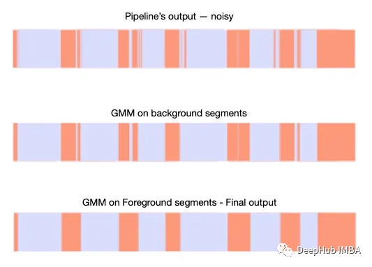
可以看到，在第一次迭代之后减少了背景类中的噪声，第二次迭代之后减少了前景类中的噪声。

结果展示

下面我们展示平滑算法的一些结果。并且还测量了信噪比(SNR)[10]，得到了一些数值结果来评估算法。比较平滑前后，对前景类和背景类进行了两次信噪比。这里的淡紫色部分代表前景部分，橙色部分代表背景部分。

总结

在本文中探讨GMM作为时间数据平滑算法的使用。GMM（Gaussian Mixture Model）是一种统计模型，常用于数据聚类和密度估计。虽然它主要用于聚类任务，但也可以在一定程度上用作时间数据平滑算法。虽然它并不是专门为此任务设计的，但是对于这种类别相关的数据平滑，GMM在降噪和结果改善方面表现非常好（信噪比参数）。

引用：

[1] Girshick, R., Donahue, J., Darrell, T. and Malik, J., 2014. Rich feature hierarchies for accurate object detection and semantic segmentation. In Proceedings of the IEEE conference on computer vision and pattern recognition (pp. 580–587).

[2] Girshick, R., 2015. Fast r-cnn. In Proceedings of the IEEE international conference on computer vision (pp. 1440–1448).

[3] Ren, S., He, K., Girshick, R. and Sun, J., 2015. Faster r-cnn: Towards real-time object detection with region proposal networks. Advances in neural information processing systems, 28.

[4] Feichtenhofer, Christoph, Haoqi Fan, Jitendra Malik, and Kaiming He. “Slowfast networks for video recognition.” In Proceedings of the IEEE/CVF international conference on computer vision, pp. 6202–6211. 2019.

[5] Normal distribution, *Wikipedia,*https://en.wikipedia.org/wiki/Normal_distribution

[6] Normal Distribution, Feldman K., https://www.isixsigma.com/dictionary/normal-distribution/

[7] Scikit-learn: Machine Learning in Python, Pedregosa, et al., JMLR 12, pp. 2825–2830, 2011.

[8] Reynolds, D.A., 2009. Gaussian mixture models. Encyclopedia of biometrics, 741(659–663).

[9] Kireeva A., 2001, Gaussian Mixture Models Visually Explained, https://aabkn.github.io/GMM_visually_explained

[10] Signal-to-noise ratio, *Wikipedia,*https://en.wikipedia.org/wiki/Signal-to-noise_ratio

作者：Tal Goldfryd

标签：机器学习 GMM 时间序列

基于GMM的一维时序数据平滑算法

高斯混合模型

基于 GMM 的平滑器

代码和解释

结果展示

总结

发表评论

“基于GMM的一维时序数据平滑算法”的评论:

关于作者

Deephub

相关阅读

文章导航