
本文将对Self-Training的流程做一个详细的介绍并使用Python 和Sklearn 实现一个完整的Self-Training示例。
半监督学习结合了标记和未标记的数据,可以扩展模型训练时可用的数据池。我们无需手动标记数千个示例,就可以提高模型性能并节省大量时间和金钱。
如果你经常使用有监督的机器学习算法,你肯定会很高兴听到:可以通过一种称为Self-Training的技术快速调整模型的训练方法并享受到半监督方法的好处。
Self-Training属于机器学习算法的半监督分支,因为它使用标记和未标记数据的组合来训练模型。
Self-Training是如何进行的?
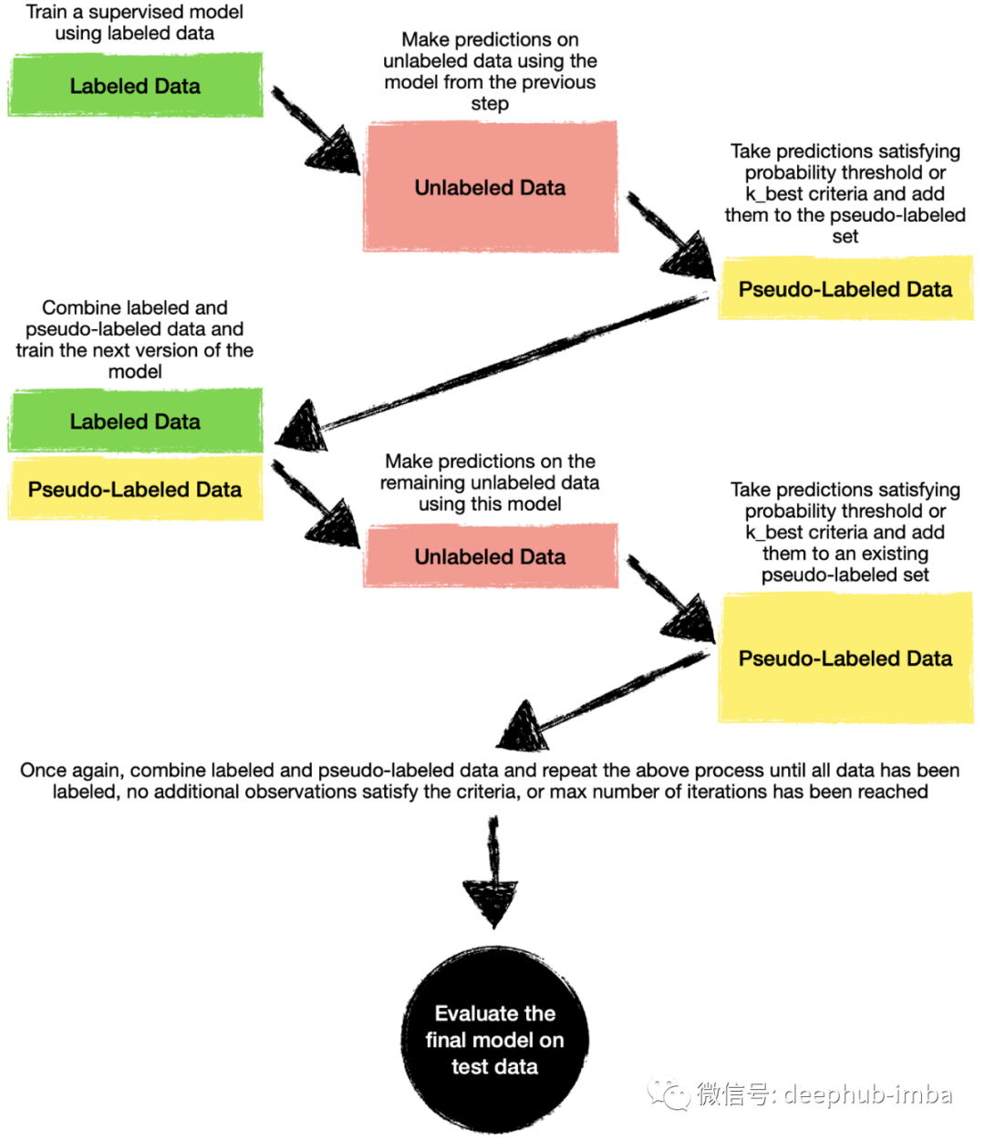
你可能认为Self-Training包含一些魔法或者是一个高度复杂的方法。其实Self-Training背后的想法非常的简单,可以通过以下步骤来解释:
- 收集所有标记和未标记的数据,但我们只使用标记的数据来训练我们的第一个监督模型。
- 利用该模型预测未标记数据的类别。
- 选择满足预定义标准的观测结果(例如,预测概率为>90%或属于预测概率最高的前10个观测结果),并将这些伪标签与标记数据结合起来。
- 通过使用标签和伪标签来训练一个新的监督模型。然后我们再次进行预测,并将新观察结果添加到伪标记池中。
- 我们迭代这些步骤,当没有其他未标记的观测满足伪标记标准,或者达到指定的最大迭代次数时,迭代结束。
下面是我刚才描述的所有步骤的总结:
如何在 Python 中使用Self-Training?
现在让我们通过一个 Python 示例对现实数据使用Self-Training技术进行训练
我们将使用以下数据和库:
- 来自 Kaggle 的营销活动数据
- Scikit-learn 库:train_test_split、SelfTrainingClassifier、classification_report
- 用于数据可视化的 Plotly
- 用于数据操作的 Pandas
# Data manipulation
import pandas as pd

# Visualization
import plotly.express as px

# Sklearn
from sklearn.model_selection import train_test_split # for splitting data into train and test samples
from sklearn.svm import SVC # for Support Vector Classification baseline model
from sklearn.semi_supervised import SelfTrainingClassifier # for Semi-Supervised learning
from sklearn.metrics import classification_report # for model evaluation metrics
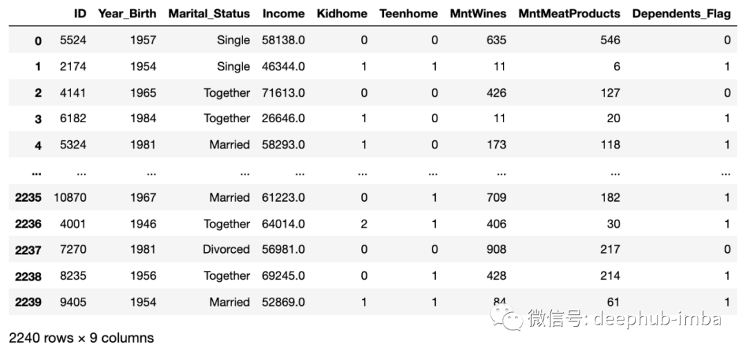
接下来,我们下载并获取数据。这里将文件限制在几个关键列,因为我们将只使用两个特征来训练我们的示例模型。
# Read in data
df = pd.read_csv('marketing_campaign.csv',
                 encoding='utf-8', delimiter=';',
                 usecols=['ID', 'Year_Birth', 'Marital_Status', 'Income', 'Kidhome', 'Teenhome', 'MntWines', 'MntMeatProducts']
                )

# Create a flag to denote whether the person has any dependants at home (either kids or teens)
df['Dependents_Flag']=df.apply(lambda x: 1 if x['Kidhome']+x['Teenhome']>0 else 0, axis=1)

# Print dataframe
df
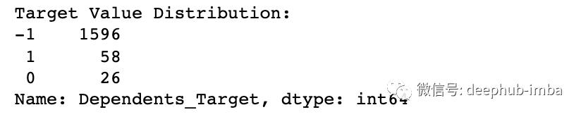
“Dependents_Flag”是我们预测的目标:预测我们的超市购物者是否在家中有小孩(儿童/青少年)。
这就是数据的样子:
在开始训练模型之前,我们还需要做一些事情。由于我们的目标是训练和评估Self-Training(一种半监督技术)的性能,因此我们将按照以下设置拆分数据。
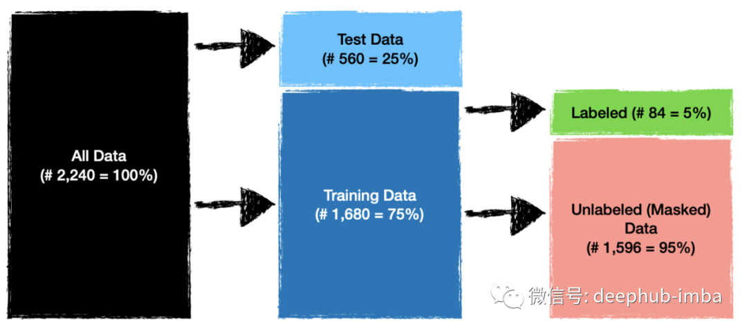
测试数据将用于评估模型性能,而标记和未标记的数据将用于训练我们的模型。让我们将数据拆分为训练样本和测试样本并打印形状以检查大小是否正确:
df_train, df_test = train_test_split(df, test_size=0.25, random_state=0)
print('Size of train dataframe: ', df_train.shape[0])
print('Size of test dataframe: ', df_test.shape[0])

现在让我们在训练数据中屏蔽95%的标签,并创建一个目标变量,使用' -1 '表示未标记(屏蔽)数据:
# Create a flag for label masking
df_train['Random_Mask'] = True
df_train.loc[df_train.sample(frac=0.05, random_state=0).index, 'Random_Mask'] = False

# Create a new target colum with labels. The 1's and 0's are original labels and -1 represents unlabeled (masked) data
df_train['Dependents_Target']=df_train.apply(lambda x: x['Dependents_Flag'] if x['Random_Mask']==False else -1, axis=1)

# Show target value distribution
print('Target Value Distribution:')
print(df_train['Dependents_Target'].value_counts())
在训练开始之前,使用二维散点图,看看数据是如何分布的。
# Create a scatter plot
fig = px.scatter(df_train, x='MntMeatProducts', y='MntWines', opacity=1, color=df_train['Dependents_Target'].astype(str),
                 color_discrete_sequence=['lightgrey', 'red', 'blue'],
                )

# Change chart background color
fig.update_layout(dict(plot_bgcolor = 'white'))

# Update axes lines
fig.update_xaxes(showgrid=True, gridwidth=1, gridcolor='white',
                 zeroline=True, zerolinewidth=1, zerolinecolor='white',
                 showline=True, linewidth=1, linecolor='white')

fig.update_yaxes(showgrid=True, gridwidth=1, gridcolor='white',
                 zeroline=True, zerolinewidth=1, zerolinecolor='white',
                 showline=True, linewidth=1, linecolor='white')

# Set figure title
fig.update_layout(title_text="Marketing Campaign Training Data - Labeled vs. Unlabeled")

# Update marker size
fig.update_traces(marker=dict(size=5))

fig.show()
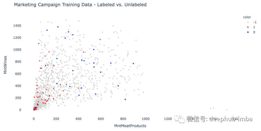
我们将使用“MntMeatProducts”(购物者在肉制品上的年度支出)和“MntWines”(购物者在葡萄酒上的年度支出)作为两个特征来进行训练。
模型训练
现在数据已经准备好,我们将在标记数据上训练一个有监督的支持向量机分类模型(SVC),并将它作为性能测试的基线模型,这样我们能够从后面的步骤判断半监督方法比标准监督模型更好还是更差。
########## Step 1 - Data Prep ##########
# Select only records with known labels
df_train_labeled=df_train[df_train['Dependents_Target']!=-1]

# Select data for modeling
X_baseline=df_train_labeled[['MntMeatProducts', 'MntWines']]
y_baseline=df_train_labeled['Dependents_Target'].values

# Put test data into an array
X_test=df_test[['MntMeatProducts', 'MntWines']]
y_test=df_test['Dependents_Flag'].values

########## Step 2 - Model Fitting ##########
# Specify SVC model parameters
model = SVC(kernel='rbf',
            probability=True,
            C=1.0, # default = 1.0
            gamma='scale', # default = 'scale'
            random_state=0
           )

# Fit the model
clf = model.fit(X_baseline, y_baseline)

########## Step 3 - Model Evaluation ##########
# Use score method to get accuracy of the model
print('---------- SVC Baseline Model - Evaluation on Test Data ----------')
accuracy_score_B = model.score(X_test, y_test)
print('Accuracy Score: ', accuracy_score_B)
# Look at classification report to evaluate the model
print(classification_report(y_test, model.predict(X_test)))
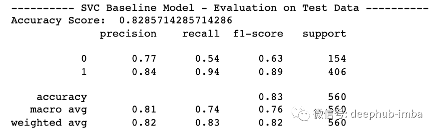
有监督的 SVC 模型的结果已经相当不错,准确率为 82.85%。由于类别不平衡,label=1(有小孩的购物者)的 f1 分数更高。
现在让我们使用 Sklearn 的SelfTrainingClassifier,同时使用相同的 SVC 模型作为基础估计器。作为Sklearn的一部分SelfTrainingClassifier支持与任何兼容sklearn标准的分类模型进行整合。
########## Step 1 - Data Prep ##########
# Select data for modeling - we are including masked (-1) labels this time
X_train=df_train[['MntMeatProducts', 'MntWines']]
y_train=df_train['Dependents_Target'].values

########## Step 2 - Model Fitting ##########
# Specify SVC model parameters
model_svc = SVC(kernel='rbf',
                probability=True, # Need to enable to be able to use predict_proba
                C=1.0, # default = 1.0
                gamma='scale', # default = 'scale',
                random_state=0
               )

# Specify Self-Training model parameters
self_training_model = SelfTrainingClassifier(base_estimator=model_svc, # An estimator object implementing fit and predict_proba.
                                             threshold=0.7, # default=0.75, The decision threshold for use with criterion='threshold'. Should be in [0, 1).
                                             criterion='threshold', # {‘threshold’, ‘k_best’}, default=’threshold’, The selection criterion used to select which labels to add to the training set. If 'threshold', pseudo-labels with prediction probabilities above threshold are added to the dataset. If 'k_best', the k_best pseudo-labels with highest prediction probabilities are added to the dataset.
                                             #k_best=50, # default=10, The amount of samples to add in each iteration. Only used when criterion='k_best'.
                                             max_iter=100, # default=10, Maximum number of iterations allowed. Should be greater than or equal to 0. If it is None, the classifier will continue to predict labels until no new pseudo-labels are added, or all unlabeled samples have been labeled.
                                             verbose=True # default=False, Verbosity prints some information after each iteration
                                            )

# Fit the model
clf_ST = self_training_model.fit(X_train, y_train)

########## Step 3 - Model Evaluation ##########
print('')
print('---------- Self Training Model - Summary ----------')
print('Base Estimator: ', clf_ST.base_estimator_)
print('Classes: ', clf_ST.classes_)
print('Transduction Labels: ', clf_ST.transduction_)
#print('Iteration When Sample Was Labeled: ', clf_ST.labeled_iter_)
print('Number of Features: ', clf_ST.n_features_in_)
print('Feature Names: ', clf_ST.feature_names_in_)
print('Number of Iterations: ', clf_ST.n_iter_)
print('Termination Condition: ', clf_ST.termination_condition_)
print('')

print('---------- Self Training Model - Evaluation on Test Data ----------')
accuracy_score_ST = clf_ST.score(X_test, y_test)
print('Accuracy Score: ', accuracy_score_ST)
# Look at classification report to evaluate the model
print(classification_report(y_test, clf_ST.predict(X_test)))
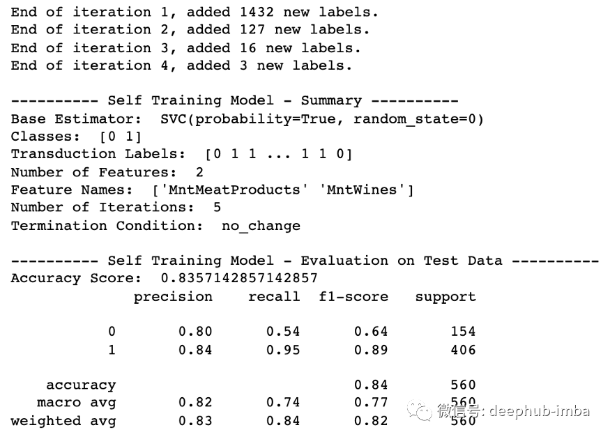
结果出来了!模型性能的确提高了,虽然只是略微提高到 83.57% 的准确率。由于精度提高,标签=0 的 F1 分数也略好一些。
正如文章前面提到的,我们可以设定如何选择伪标签的规则。例如可以基于前 k_best 预测或指定特定的概率阈值。
在这个例子中,使用了 0.7 的概率阈值。这意味着任何类别概率为 0.7 或更高的观测值都将被添加到伪标记数据池中,并用于在下一次迭代中训练模型。
阈值和 k_best可以看作Self-Training的超参数,可以设定不同的值来确认哪种设置产生最佳结果(我在本示例中没有这样做)。
总结
Self-Training可以用半监督的方式对任何监督分类算法进行训练。如果有大量未标记的数据,建议在进行昂贵的数据标记练习之前先尝试以下半监督学习。
作者:Saul Dobilas