机器学习与深度学习——通过knn算法分类鸢尾花数据集iris求出错误率并进行可视化

什么是knn算法？

KNN算法是一种基于实例的机器学习算法，其全称为K-最近邻算法（K-Nearest Neighbors Algorithm）。它是一种简单但非常有效的分类和回归算法。
该算法的基本思想是：对于一个新的输入样本，通过计算它与训练集中所有样本的距离，找到与它距离最近的K个训练集样本，然后基于这K个样本的类别信息来进行分类或回归预测。KNN算法中的“K”代表了在预测时使用的邻居数，通常需要手动设置。
KNN算法的主要优点是简单、易于实现，并且在某些情况下可以获得很好的分类或回归精度。但是，它也有一些缺点，如需要存储所有训练集样本、计算距离的开销较大、对于高维数据容易过拟合等。

KNN算法常用于分类问题，如文本分类、图像分类等，以及回归问题，如预测房价等。

我们这次学习机器学习的knn算法分别对前二维数据和前四维数据进行训练和可视化。

两个目标：

1、通过knn算法对iris数据集前两个维度的数据进行模型训练并求出错误率，最后进行可视化展示数据区域划分。
2、通过knn算法对iris数据集总共四个维度的数据进行模型训练并求出错误率，并对前四维数据进行可视化。

基本思路：

1、先载入iris数据集 Load Iris data
2、分离训练集和设置测试集split train and test sets
3、对数据进行标准化处理Normalize the data
4、使用knn模型进行训练Train using KNN
5、然后进行可视化处理Visualization
6、最后通过绘图决策平面plot decision plane

1、通过knn算法对iris数据集前两个维度的数据进行模型训练并求出错误率，最后进行可视化展示数据区域划分：

from sklearn import datasets
import numpy as np
### Load Iris data
iris = datasets.load_iris()
x = iris.data[:,:2]#前2个维度# x = iris.data
y = iris.target
print("class labels: ", np.unique(y))
x.shape
y.shape
### split train and test sets
from sklearn.model_selection import train_test_split
x_train, x_test, y_train, y_test = train_test_split(x, y, test_size=0.2, stratify=y)
x_train.shape
print("Labels count in y:", np.bincount(y))
print("Labels count in y_train:", np.bincount(y_train))
print("Labels count in y_test:", np.bincount(y_test))### Normalize the data
from sklearn.preprocessing import StandardScaler
sc = StandardScaler()
sc.fit(x_train)
x_train_std = sc.transform(x_train)
x_test_std = sc.transform(x_test)
print("TrainSets Orig mean:{}, std mean:{}".format(np.mean(x_train,axis=0), np.mean(x_train_std,axis=0)))
print("TrainSets Orig std:{}, std std:{}".format(np.std(x_train,axis=0), np.std(x_train_std,axis=0)))
print("TestSets Orig mean:{}, std mean:{}".format(np.mean(x_test,axis=0), np.mean(x_test_std,axis=0)))
print("TestSets Orig std:{}, std std:{}".format(np.std(x_test,axis=0), np.std(x_test_std,axis=0)))### Train using KNN
from sklearn.neighbors import KNeighborsClassifier
knn = KNeighborsClassifier(n_neighbors=5, p=2, metric='minkowski')
knn.fit(x_train_std, y_train)pred_test=knn.predict(x_test_std)
err_num =(pred_test != y_test).sum()
rate = err_num/y_test.size
print("Misclassfication num: {}\nError rate: {}".format(err_num, rate))#计算错误率### Visualization
x_combined_std = np.vstack((x_train_std, x_test_std))
y_combined = np.hstack((y_train, y_test))
plot_decision_regions(x_combined_std, y_combined,
classifier=knn, test_idx=range(105,150))
plt.xlabel('petal length [standardized]')
plt.ylabel('petal width [standardized]')
plt.legend(loc='upper left')
plt.tight_layout()
plt.show()#### plot decision plane
x_combined_std = np.vstack((x_train_std, x_test_std))
y_combined = np.hstack((y_train, y_test))
plot_decision_regions(x_combined_std, y_combined,
classifier=knn, test_idx=range(105,150))
plt.xlabel('petal length [standardized]')
plt.ylabel('petal width [standardized]')
plt.legend(loc='upper left')
plt.tight_layout()
plt.show()

代码及其可视化效果截图：

2、通过knn算法对iris数据集总共四个维度的数据进行模型训练并求出错误率并进行可视化：

from sklearn import datasets
import numpy as np
iris = datasets.load_iris()
x = iris.data  #4个维度# x = iris.data
y = iris.target
print("class labels: ", np.unique(y))
x.shape
y.shape
### split train and test sets
from sklearn.model_selection import train_test_split
x_train, x_test, y_train, y_test = train_test_split(x, y, test_size=0.2, stratify=y)
x_train.shape
print("Labels count in y:", np.bincount(y))
print("Labels count in y_train:", np.bincount(y_train))
print("Labels count in y_test:", np.bincount(y_test))### Normalize the data
from sklearn.preprocessing import StandardScaler
sc = StandardScaler()
sc.fit(x_train)
x_train_std = sc.transform(x_train)
x_test_std = sc.transform(x_test)
print("TrainSets Orig mean:{}, std mean:{}".format(np.mean(x_train,axis=0), np.mean(x_train_std,axis=0)))
print("TrainSets Orig std:{}, std std:{}".format(np.std(x_train,axis=0), np.std(x_train_std,axis=0)))
print("TestSets Orig mean:{}, std mean:{}".format(np.mean(x_test,axis=0), np.mean(x_test_std,axis=0)))
print("TestSets Orig std:{}, std std:{}".format(np.std(x_test,axis=0), np.std(x_test_std,axis=0)))### Train using KNN
from sklearn.neighbors import KNeighborsClassifier
knn = KNeighborsClassifier(n_neighbors=5, p=2, metric='minkowski')
knn.fit(x_train_std, y_train)pred_test=knn.predict(x_test_std)
err_num =(pred_test != y_test).sum()
rate = err_num/y_test.size
print("Misclassfication num: {}\nError rate: {}".format(err_num, rate))#计算错误率#四维可视化在二维或三维空间中是无法呈现的，但我们可以使用降维技术来可视化数据。在这种情况下，我们可以使用主成分分析（PCA）或线性判别分析（LDA）等技术将数据降到二维或三维空间中，并在此空间中可视化数据。import matplotlib.pyplot as plt
from mpl_toolkits.mplot3d import Axes3D
from sklearn.decomposition import PCA
# Perform PCA to reduce the dimensionality from 4D to 3D
pca = PCA(n_components=3)
x_train_pca = pca.fit_transform(x_train_std)# Create a 3D plot of the first three principal components
fig = plt.figure(figsize=(8, 8))
ax = fig.add_subplot(111, projection='3d')# Plot the three classes in different colorsfor label, color in zip(np.unique(y_train), ['blue', 'red', 'green']):
    ax.scatter(x_train_pca[y_train==label, 0], 
               x_train_pca[y_train==label, 1], 
               x_train_pca[y_train==label, 2], 
               c=color, label=label, alpha=0.8)
ax.set_xlabel('PC1')
ax.set_ylabel('PC2')
ax.set_zlabel('PC3')
ax.legend(loc='upper right')
ax.set_title('Iris Dataset - PCA')
plt.show()

四维可视化在二维或三维空间中是无法呈现的，但我们可以使用降维技术来可视化数据。在这种情况下，我们可以使用主成分分析（PCA）或线性判别分析（LDA）等技术将数据降到二维或三维空间中，并在此空间中可视化数据。
下面是代码效果图，展示如何使用PCA将四维数据降至三维，并在三维空间中可视化iris数据集：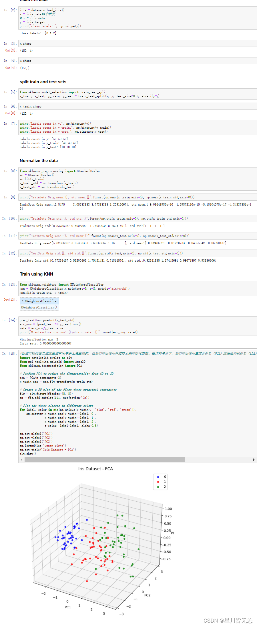

将iris数据集的四维数据降至三维，并在三维空间中可视化了训练集。每个点代表一个数据样本，不同颜色代表不同的类别。我们可以看到，在三维空间中，有两个类别可以相对清晰地分开，而另一个类别则分布在两个主成分的中间。

我们要注意对于高维数据使用knn算法容易出现高维数据容易过拟合的情况，这是因为在高维空间中，数据点之间的距离变得很大，同时训练样本的数量相对于特征的数量很少，容易导致KNN算法无法很好地进行预测。

为了避免高维数据容易过拟合的情况，可以采取以下措施：

1. 特征选择：选择有意义的特征进行训练，可以降低特征数量，避免过拟合。常用的特征选择方法有Filter方法、Wrapper方法和Embedded方法。
2. 降维：可以通过主成分分析（PCA）等方法将高维数据映射到低维空间中，以减少特征数量，避免过拟合。
3. 调整K值：KNN算法中的K值决定了邻居的数量，K值过大容易出现欠拟合，而K值过小容易出现过拟合。因此，可以通过交叉验证等方法来确定最佳的K值。
4. 距离度量：KNN算法中的距离度量方法对结果影响较大，不同的距离度量方法会导致不同的预测结果。因此，可以尝试不同的距离度量方法，选择最优的方法。
5. 数据增强：在数据量较少的情况下，可以通过数据增强的方法来增加训练样本，以提高模型的泛化能力。

希望通过这片文章能够进一步认识knn算法的原理及其应用。
今天是五一劳动节，在这里小马同学祝各位五一劳动节快乐！