
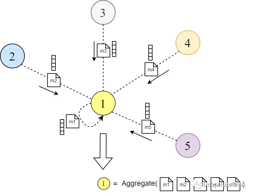
图神经网络(gnn)是一类功能强大的神经网络,它对图结构数据进行操作。它们通过从节点的局部邻域聚合信息来学习节点表示(嵌入)。这个概念在图表示学习文献中被称为“消息传递”。
消息(嵌入)通过多个GNN层在图中的节点之间传递。每个节点聚合来自其邻居的消息以更新其表示。这个过程跨层重复,允许节点获得编码有关图的更丰富信息的表示。gnn的一主要变体有GraphSAGE[2]、Graph Convolution Network[3]等。
图注意力网络(GAT)[1]是一类特殊的gnn,主要的改进是消息传递的方式。他们引入了一种可学习的注意力机制,通过在每个源节点和目标节点之间分配权重,使节点能够在聚合来自本地邻居的消息时决定哪个邻居节点更重要,而不是以相同的权重聚合来自所有邻居的信息。
图注意力网络在节点分类、链接预测和图分类等任务上优于许多其他GNN模型。他们在几个基准图数据集上也展示了最先进的性能。
在这篇文章中,我们将介绍原始“Graph Attention Networks”(by Veličković )论文的关键部分,并使用PyTorch实现论文中提出的概念,这样以更好地掌握GAT方法。
论文引言
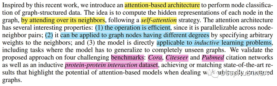
在第1节“引言”中对图表示学习文献中的现有方法进行了广泛的回顾之后,论文介绍了图注意网络(GAT)。
然后将论文的方法与现有的一些方法进行比较,并指出它们之间的一般异同,这是论文的常用格式,就不多介绍了。
GAT的架构
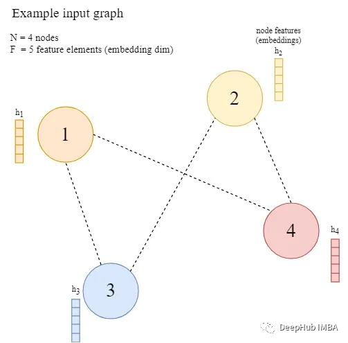
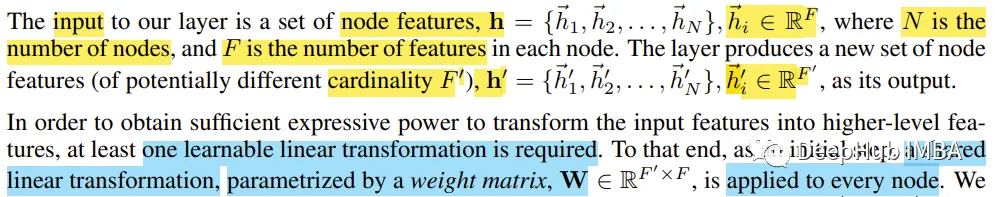
本节是本文的主要部分,对图注意力网络的体系结构进行了详细的阐述。为了进一步解释,假设所提出的架构在一个有N个节点的图上执行(V = {V′};i=1,…,N),每个节点用向量h ^ (F个元素)表示,节点之间存在任意边。
作者首先描述了单个图注意力层的特征,以及它是如何运作的(因为它是图注意力网络的基本构建块)。一般来说,单个GAT层应该将具有给定节点嵌入(表示)的图作为输入,将信息传播到本地邻居节点,并输出更新后的节点表示。
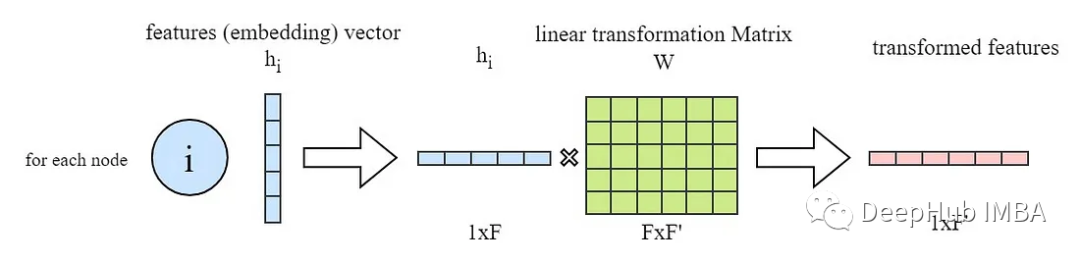
如上所述,ga层的所有输入节点特征向量(h′)都是线性变换的(即乘以一个权重矩阵W),在PyTorch中,通常是这样做的:
 import torch
 from torch import nn

 # in_features -> F and out_feature -> F'
 in_features = ...
 out_feature = ...

 # instanciate the learnable weight matrix W (FxF')
 W = nn.Parameter(torch.empty(size=(in_features, out_feature)))

 #  Initialize the weight matrix W
 nn.init.xavier_normal_(W)

 # multiply W and h (h is input features of all the nodes -> NxF matrix)
 h_transformed = torch.mm(h, W)
获得了输入节点特征(嵌入)的转换版本后我们先跳到最后查看和理解GAT层的最终目标是什么。
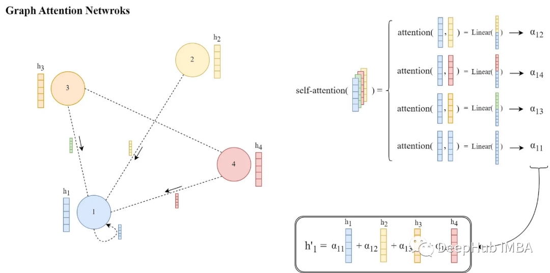
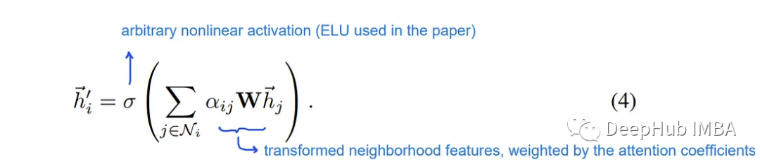
如论文所述,在图注意层的最后,对于每个节点i,我们需要从其邻域获得一个新的特征向量,该特征向量更具有结构和上下文感知性。
这是通过计算相邻节点特征的加权和,然后是非线性激活函数σ来完成的。根据Graph ML文献,这个加权和在一般GNN层操作中也被称为“聚合”步骤。
论文的这些权重α′ⱼ∈[0,1]是通过一种关注机制来学习和计算的,该机制表示在消息传递和聚合过程中节点i的邻居j特征的重要性。
每一对节点i和它的邻居j计算这些注意权值α′ⱼ的计算方法如下
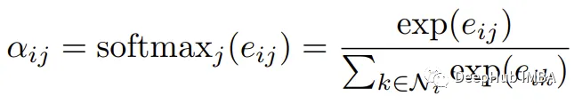
其中e ^ⱼ是注意力得分,在应用Softmax函数后,有权重都会在[0,1]区间内,并且和为1。现在通过注意函数a(…)计算每个节点i和它的邻居j∈N′之间的注意分数e′ⱼ,如下所示:
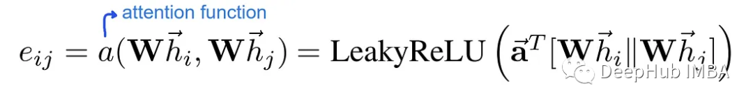
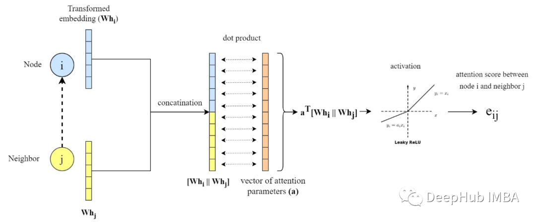
上图中的||表示两个转换后的节点嵌入的连接,a是大小为2 * F '(转换后嵌入大小的两倍)的可学习参数(即注意力参数)向量。而(a¹)是向量a的转置,导致整个表达式a¹[Wh′|| Whⱼ]是“a”与转换后的嵌入的连接之间的点(内)积。
整个操作说明如下:
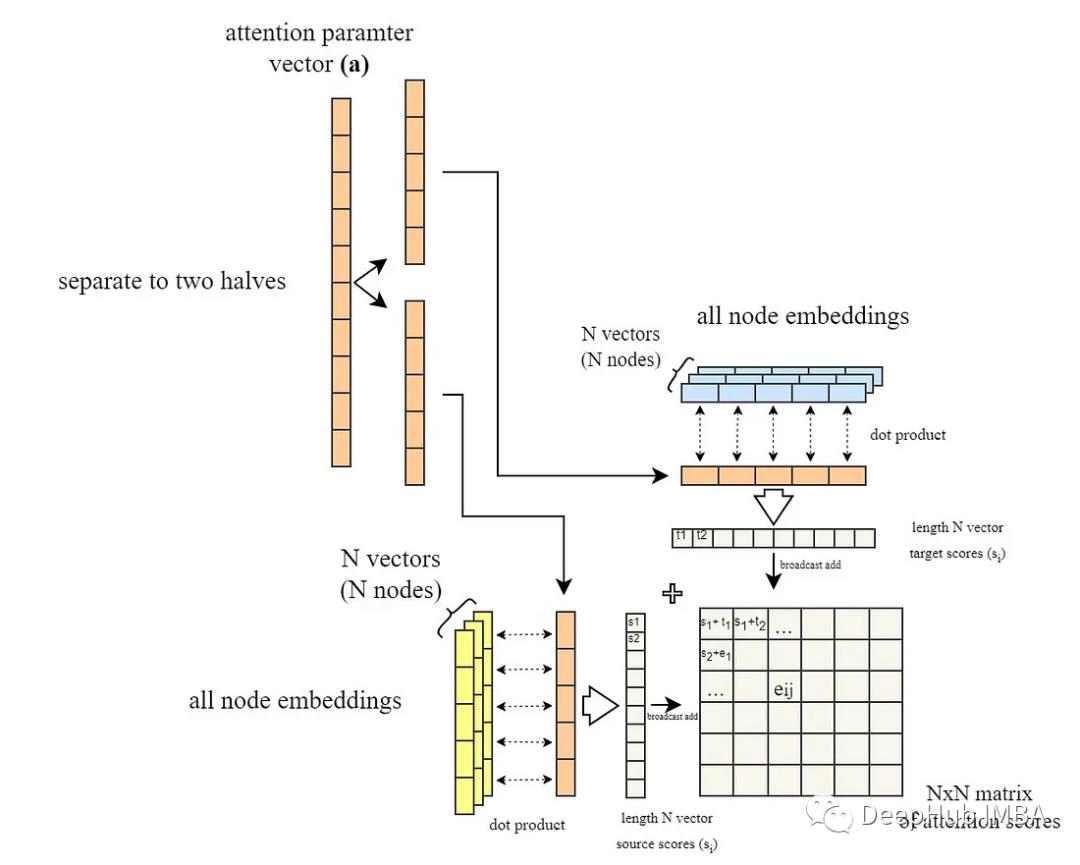
在PyTorch中,我们采用了一种稍微不同的方法。因为计算所有节点对之间的e′ⱼ然后只选择代表节点之间现有边的那些是更有效的。来计算所有的e′ⱼ
 # instanciate the learnable attention parameter vector `a`
 a = nn.Parameter(torch.empty(size=(2 * out_feature, 1)))

 # Initialize the parameter vector `a`
 nn.init.xavier_normal_(a)

 # we obtained `h_transformed` in the previous code snippet

 # calculating the dot product of all node embeddings
 # and first half the attention vector parameters (corresponding to neighbor messages)
 source_scores = torch.matmul(h_transformed, self.a[:out_feature, :])

 # calculating the dot product of all node embeddings
 # and second half the attention vector parameters (corresponding to target node)
 target_scores = torch.matmul(h_transformed, self.a[out_feature:, :])

 # broadcast add
 e = source_scores + target_scores.T
 e = self.leakyrelu(e)
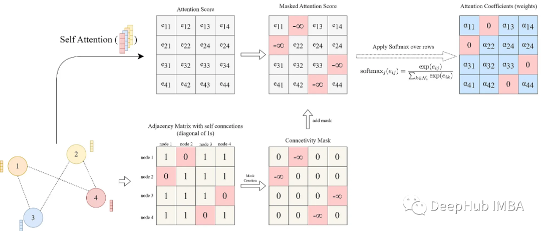
代码片段的最后一部分(# broadcast add)将所有一对一的源和目标分数相加,得到一个包含所有e′ⱼ分数的NxN矩阵。(下图所示)
到目前为止,我们假设图是完全连接的,我们计算的是所有可能的节点对之间的注意力得分。但是其实大部分情况下图不可能是完全连接的,所以为了解决这个问题,在将LeakyReLU激活应用于注意力分数之后,注意力分数基于图中现有的边被屏蔽,这意味着我们只保留与现有边对应的分数。
它可以通过给不存在边的节点之间的分数矩阵中的元素分配一个大的负分数(近似于-∞)来完成,这样它们对应的注意力权重在softmax之后变为零(还记得我们以前发的注意力掩码么,就是一样的道理)。
这里的注意力掩码是通过使用图的邻接矩阵来实现的。邻接矩阵是一个NxN矩阵,如果节点i和j之间存在一条边,则在第i行和第j列处为1,在其他地方为0。因此,我们通过将邻接矩阵的零元素赋值为-∞并在其他地方赋值为0来创建掩码。然后将掩码添加到分数矩阵中。然后在它的行上应用softmax函数。
 connectivity_mask = -9e16 * torch.ones_like(e)
 # adj_mat is the N by N adjacency matrix
 e = torch.where(adj_mat > 0, e, connectivity_mask) # masked attention scores

 # attention coefficients are computed as a softmax over the rows
 # for each column j in the attention score matrix e
 attention = F.softmax(e, dim=-1)
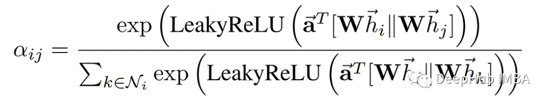
最后,根据论文描述,在获得注意力分数并将其与现有的边进行掩码遮蔽后,通过对分数矩阵的行执行softmax,得到注意力权重α¹ⱼ。
我们通过一个完整的可视化图过程如下:
最后就是计算节点嵌入的加权和:
 # final node embeddings are computed as a weighted average of the features of its neighbors
 h_prime = torch.matmul(attention, h_transformed)
以上一个一个注意力头的工作流程和原理,论文还引入了多头的概念,其中所有操作都是通过多个并行的操作流来完成的。
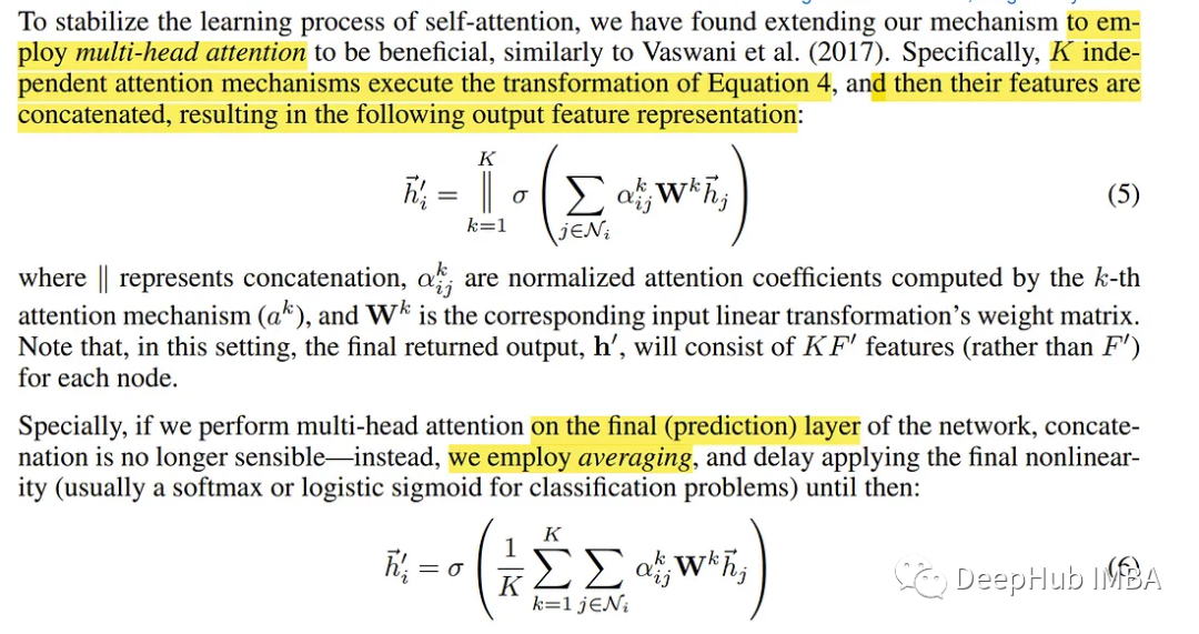
多头注意力和聚合过程如下图所示:
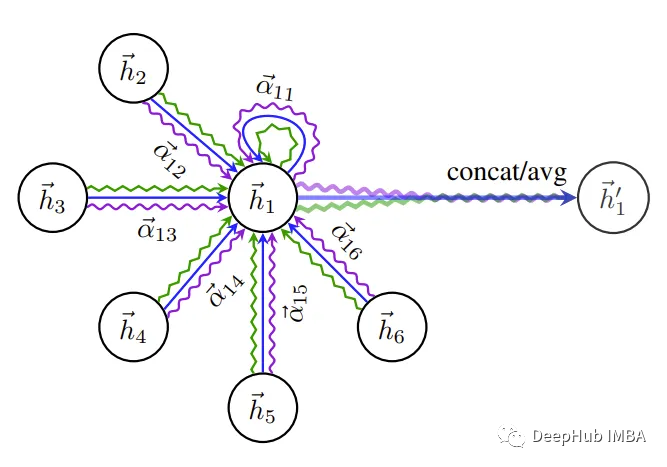
节点1在其邻域中的多头注意力(K = 3个头),不同的箭头样式和颜色表示独立的注意力计算。将来自每个头部的聚合特征连接或平均以获得h '。
为了以更简洁的模块化形式(作为PyTorch模块)封装实现并合并多头注意力的功能,整个Graph关注层的实现如下:
 import torch
 from torch import nn
 import torch.nn.functional as F

 ################################
 ###  GAT LAYER DEFINITION    ###
 ################################

 class GraphAttentionLayer(nn.Module):

     def __init__(self, in_features: int, out_features: int,
                  n_heads: int, concat: bool = False, dropout: float = 0.4,
                  leaky_relu_slope: float = 0.2):
         super(GraphAttentionLayer, self).__init__()

         self.n_heads = n_heads # Number of attention heads
         self.concat = concat # wether to concatenate the final attention heads
         self.dropout = dropout # Dropout rate

         if concat: # concatenating the attention heads
             self.out_features = out_features # Number of output features per node
             assert out_features % n_heads == 0 # Ensure that out_features is a multiple of n_heads
             self.n_hidden = out_features // n_heads
         else: # averaging output over the attention heads (Used in the main paper)
             self.n_hidden = out_features

         #  A shared linear transformation, parametrized by a weight matrix W is applied to every node
         #  Initialize the weight matrix W
         self.W = nn.Parameter(torch.empty(size=(in_features, self.n_hidden * n_heads)))

         # Initialize the attention weights a
         self.a = nn.Parameter(torch.empty(size=(n_heads, 2 * self.n_hidden, 1)))

         self.leakyrelu = nn.LeakyReLU(leaky_relu_slope) # LeakyReLU activation function
         self.softmax = nn.Softmax(dim=1) # softmax activation function to the attention coefficients

         self.reset_parameters() # Reset the parameters


     def reset_parameters(self):

         nn.init.xavier_normal_(self.W)
         nn.init.xavier_normal_(self.a)

     def _get_attention_scores(self, h_transformed: torch.Tensor):

         source_scores = torch.matmul(h_transformed, self.a[:, :self.n_hidden, :])
         target_scores = torch.matmul(h_transformed, self.a[:, self.n_hidden:, :])

         # broadcast add
         # (n_heads, n_nodes, 1) + (n_heads, 1, n_nodes) = (n_heads, n_nodes, n_nodes)
         e = source_scores + target_scores.mT
         return self.leakyrelu(e)

     def forward(self,  h: torch.Tensor, adj_mat: torch.Tensor):

         n_nodes = h.shape[0]

         # Apply linear transformation to node feature -> W h
         # output shape (n_nodes, n_hidden * n_heads)
         h_transformed = torch.mm(h, self.W)
         h_transformed = F.dropout(h_transformed, self.dropout, training=self.training)

         # splitting the heads by reshaping the tensor and putting heads dim first
         # output shape (n_heads, n_nodes, n_hidden)
         h_transformed = h_transformed.view(n_nodes, self.n_heads, self.n_hidden).permute(1, 0, 2)

         # getting the attention scores
         # output shape (n_heads, n_nodes, n_nodes)
         e = self._get_attention_scores(h_transformed)

         # Set the attention score for non-existent edges to -9e15 (MASKING NON-EXISTENT EDGES)
         connectivity_mask = -9e16 * torch.ones_like(e)
         e = torch.where(adj_mat > 0, e, connectivity_mask) # masked attention scores

         # attention coefficients are computed as a softmax over the rows
         # for each column j in the attention score matrix e
         attention = F.softmax(e, dim=-1)
         attention = F.dropout(attention, self.dropout, training=self.training)

         # final node embeddings are computed as a weighted average of the features of its neighbors
         h_prime = torch.matmul(attention, h_transformed)

         # concatenating/averaging the attention heads
         # output shape (n_nodes, out_features)
         if self.concat:
             h_prime = h_prime.permute(1, 0, 2).contiguous().view(n_nodes, self.out_features)
         else:
             h_prime = h_prime.mean(dim=0)

         return h_prime
最后将上面所有的代码整合成一个完整的GAT模型:
 class GAT(nn.Module):

     def __init__(self,
         in_features,
         n_hidden,
         n_heads,
         num_classes,
         concat=False,
         dropout=0.4,
         leaky_relu_slope=0.2):

         super(GAT, self).__init__()

         # Define the Graph Attention layers
         self.gat1 = GraphAttentionLayer(
             in_features=in_features, out_features=n_hidden, n_heads=n_heads,
             concat=concat, dropout=dropout, leaky_relu_slope=leaky_relu_slope
             )

         self.gat2 = GraphAttentionLayer(
             in_features=n_hidden, out_features=num_classes, n_heads=1,
             concat=False, dropout=dropout, leaky_relu_slope=leaky_relu_slope
             )

     def forward(self, input_tensor: torch.Tensor , adj_mat: torch.Tensor):


         # Apply the first Graph Attention layer
         x = self.gat1(input_tensor, adj_mat)
         x = F.elu(x) # Apply ELU activation function to the output of the first layer

         # Apply the second Graph Attention layer
         x = self.gat2(x, adj_mat)

         return F.softmax(x, dim=1) # Apply softmax activation function
方法对比
作者对GATs和其他一些现有GNN方法/架构进行了比较:
- 由于GATs能够计算注意力权重并并行执行局部聚合,因此它比现有的一些方法计算效率更高。
- GATs可以在聚合消息时为节点的邻居分配不同的重要性,这可以实现模型容量的飞跃并提高可解释性。
- GAT不考虑节点的完整邻域(不需要从邻域采样),也不假设节点内部有任何排序。
- 通过将伪坐标函数设置为u(x, y) = f(x)||f(y), GAT可以重新表述为MoNet的一个特定实例(Monti等人,2016),其中f(x)表示(可能是mlp转换的)节点x的特征,而||是连接;权函数为wj(u) = softmax(MLP(u))
基准测试
在论文的第三部分中,作者描述了评估GAT的基准、数据集和任务。然后,他们提出了他们对模型的评估结果。
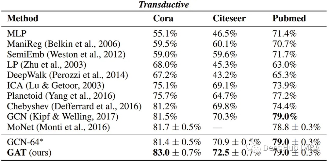
论文中用作基准的数据集分为两种类型的任务,转换和归纳。
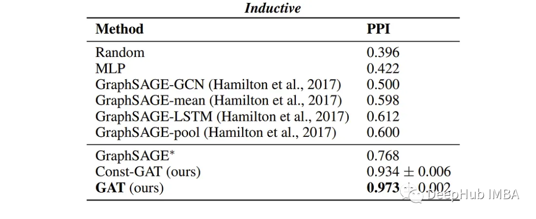
归纳学习:这是一种监督学习任务,其中模型仅在一组标记的训练样例上进行训练,并且在训练过程中完全未观察到的样例上对训练后的模型进行评估和测试。这是一种被称为普通监督学习的学习类型。
传导学习:在这种类型的任务中,所有的数据,包括训练、验证和测试实例,都在训练期间使用。但是在每个阶段,模型只访问相应的标签集。这意味着在训练期间,模型只使用由训练实例和标签产生的损失进行训练,但测试和验证特征用于消息传递。这主要是因为示例中存在的结构和上下文信息。
论文使用四个基准数据集来评估GATs,其中三个对应于传导学习,另一个用作归纳学习任务。
转导学习数据集,即Cora、Citeseer和Pubmed (Sen et al., 2008)数据集都是引文图,其中节点是已发布的文档,边(连接)是它们之间的引用,节点特征是文档的词包表示的元素。
归纳学习数据集是一个蛋白质-蛋白质相互作用(PPI)数据集,其中包含不同人体组织的图形(Zitnik & Leskovec, 2017)。数据集的详细描述如下:
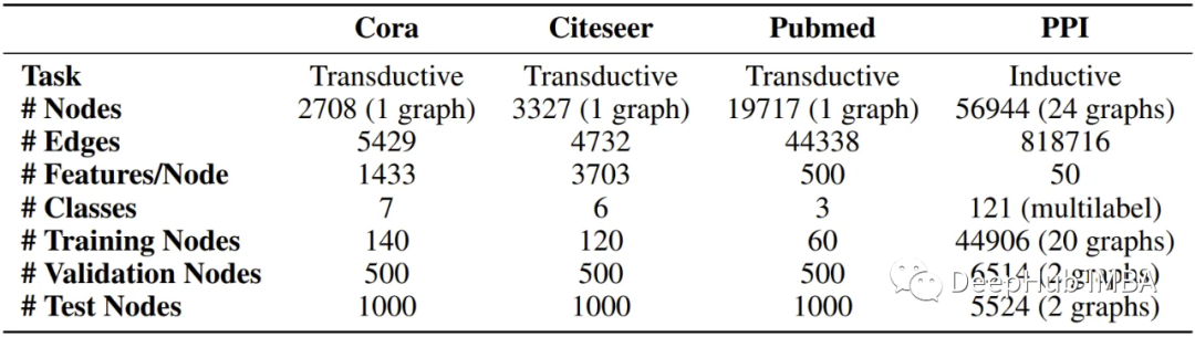
作者报告了四个基准测试的以下性能,显示了GATs与现有GNN方法的可比结果。
总结
通过阅读这篇文章并试用代码,希望你能够对GATs的工作原理以及如何在实际场景中应用它们有一个扎实的理解。
本文的完整代码在这里:
https://github.com/ebrahimpichka/GAT-pt
最后还有引用
[1] — Graph Attention Networks (2017), Petar Veličković, Guillem Cucurull, Arantxa Casanova, Adriana Romero, Pietro Liò, Yoshua Bengio. arXiv:1710.10903v3
[2] — Inductive Representation Learning on Large Graphs (2017), William L. Hamilton, Rex Ying, Jure Leskovec. arXiv:1706.02216v4
[3] — Semi-Supervised Classification with Graph Convolutional Networks (2016), Thomas N. Kipf, Max Welling. arXiv:1609.02907v4
作者:Ebrahim Pichka