
本文将使用 Python 实现和对比解释 NLP中的3 种不同文本摘要策略:老式的 TextRank(使用 gensim)、著名的 Seq2Seq(使基于 tensorflow)和最前沿的 BART(使用Transformers )。
NLP(自然语言处理)是人工智能领域,研究计算机与人类语言之间的交互,特别是如何对计算机进行编程以处理和分析大量自然语言数据。最难的 NLP 任务是输出不是单个标签或值(如分类和回归),而是完整的新文本(如翻译、摘要和对话)的任务。
文本摘要是在不改变其含义的情况下减少文档的句子和单词数量的问题。有很多不同的技术可以从原始文本数据中提取信息并将其用于摘要模型,总体来说它们可以分为提取式(Extractive)和抽象式(Abstractive)。提取方法选择文本中最重要的句子(不一定理解含义),因此作为结果的摘要只是全文的一个子集。而抽象模型使用高级 NLP(即词嵌入)来理解文本的语义并生成有意义的摘要。抽象技术很难从头开始训练,因为它们需要大量参数和数据,所以一般情况下都是用与训练的嵌入进行微调。
本文比较了 TextRank(Extractive)的老派方法、流行的编码器-解码器神经网络 Seq2Seq(Abstractive)以及彻底改变 NLP 领域的最先进的基于注意力的 Transformers(Abstractive)。
本文将使用“CNN DailyMail”数据集,包含了数千篇由 CNN 和《每日邮报》的记者用英语撰写的新闻文章,以及每篇文章的摘要,数据集和本文的代码也都会在本文末尾提供。
首先,我需要导入以下库:
## for data
import datasets  #(1.13.3)
import pandas as pd  #(0.25.1)
import numpy  #(1.16.4)

## for plotting
import matplotlib.pyplot as plt  #(3.1.2)
import seaborn as sns  #(0.9.0)

## for preprocessing
import re
import nltk  #(3.4.5)
import contractions  #(0.0.18)

## for textrank
import gensim  #(3.8.1)

## for evaluation
import rouge  #(1.0.0)
import difflib

## for seq2seq
from tensorflow.keras import callbacks, models, layers, preprocessing as kprocessing #(2.6.0)

## for bart
import transformers  #(3.0.1)
然后我使用 HuggingFace 的加载数据集:
## load the full dataset of 300k articles
dataset = datasets.load_dataset("cnn_dailymail", '3.0.0')
lst_dics = [dic for dic in dataset["train"]]

## keep the first N articles if you want to keep it lite
dtf = pd.DataFrame(lst_dics).rename(columns={"article":"text",
      "highlights":"y"})[["text","y"]].head(20000)
dtf.head()
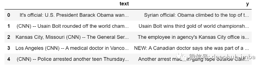
让我们检查一个随机的样本:
i = 1
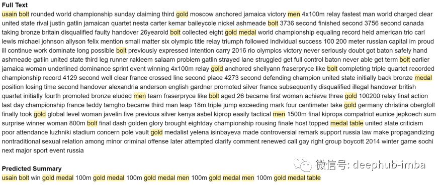
print("--- Full text ---")
print(dtf["text"][i])
print("--- Summary ---")
print(dtf["y"][i])

在上图中,我将摘要中提到的信息手动标记为红色。 体育文章对机器来说是非常困难的,因为标题需要在有限的字符限制的情况下突出主要结果。 这个实例可能是一个非常好的例子,我会将这个示例保留在测试集中以比较模型。
dtf_train = dtf.iloc[i+1:]
dtf_test = dtf.iloc[:i+1]
TextRank
TextRank (2004) 是一种基于图的文本处理排名模型,基于 Google 的 PageRank 算法,可在文本中找到最相关的句子。 PageRank 是 1998 年 Google 搜索引擎使用的第一个对网页进行排序的算法。简而言之,如果页面 A 链接到页面 B,页面 C,页面 B 链接到页面 C,那么排序将是页面 C,页面 B,页面 A。

TextRank 非常易于使用,因为它是无监督的。 首先,将整个文本拆分为句子,然后算法会使用其中句子作为节点,重叠的单词作为连接,构建一个图,通过PageRank 确定了这个句子网络中最重要的节点。
这里使用 gensim 库的内置TextRank 算法实现:
def textrank(corpus, ratio=0.2):
    if type(corpus) is str:
       corpus = [corpus]
    lst_summaries = [gensim.summarization.summarize(txt,
                     ratio=ratio) for txt in corpus]
return lst_summaries

predicted = textrank(corpus=dtf_test["text"], ratio=0.2)
predicted[i]

我们如何评估这个结果? 通常两种方式:
1、ROUGE 指标(Recall-Oriented Understudy for Gisting Evaluation):通过重叠 n-gram 将自动生成的摘要与参考摘要进行比较。
def evaluate_summary(y_test, predicted):
   rouge_score = rouge.Rouge()
   scores = rouge_score.get_scores(y_test, predicted, avg=True)
   score_1 = round(scores['rouge-1']['f'], 2)
   score_2 = round(scores['rouge-2']['f'], 2)
   score_L = round(scores['rouge-l']['f'], 2)
   print("rouge1:", score_1, "| rouge2:", score_2, "| rougeL:",
         score_2, "--> avg rouge:", round(np.mean(
         [score_1,score_2,score_L]), 2))

## Apply the function to predicted
i = 5
evaluate_summary(dtf_test["y"][i], predicted[i])

结果表明,31% 的ROUGE-1 和 7% 的ROUGE-2出现在两个摘要中,而最长的公共子序列 (ROUGE-L) 匹配了 7%。 总体而言,平均得分为 20%。 这里需要说明的是ROUGE 分数并不能衡量摘要的流畅程度,因为对于流畅程度来说我们通常使用人肉判断。
2、可视化:显示2个文本,即摘要和原文或预测摘要和真实摘要,并突出匹配部分
#Find the matching substrings in 2 strings.
def utils_split_sentences(a, b):
    ## find clean matches
    match = difflib.SequenceMatcher(isjunk=None, a=a, b=b, autojunk=True)
    lst_match = [block for block in match.get_matching_blocks() if block.size > 20]

    ## difflib didn't find any match
    if len(lst_match) == 0:
        lst_a, lst_b = nltk.sent_tokenize(a), nltk.sent_tokenize(b)

    ## work with matches
    else:
        first_m, last_m = lst_match[0], lst_match[-1]

        ### a
        string = a[0 : first_m.a]
        lst_a = [t for t in nltk.sent_tokenize(string)]
        for n in range(len(lst_match)):
            m = lst_match[n]
            string = a[m.a : m.a+m.size]
            lst_a.append(string)
            if n+1 < len(lst_match):
                next_m = lst_match[n+1]
                string = a[m.a+m.size : next_m.a]
                lst_a = lst_a + [t for t in nltk.sent_tokenize(string)]
            else:
                break
        string = a[last_m.a+last_m.size :]
        lst_a = lst_a + [t for t in nltk.sent_tokenize(string)]

        ### b
        string = b[0 : first_m.b]
        lst_b = [t for t in nltk.sent_tokenize(string)]
        for n in range(len(lst_match)):
            m = lst_match[n]
            string = b[m.b : m.b+m.size]
            lst_b.append(string)
            if n+1 < len(lst_match):
                next_m = lst_match[n+1]
                string = b[m.b+m.size : next_m.b]
                lst_b = lst_b + [t for t in nltk.sent_tokenize(string)]
            else:
                break
        string = b[last_m.b+last_m.size :]
        lst_b = lst_b + [t for t in nltk.sent_tokenize(string)]

    return lst_a, lst_b

 #Highlights the matched strings in text.
 def display_string_matching(a, b, both=True, sentences=True, titles=[]):
    if sentences is True:
        lst_a, lst_b = utils_split_sentences(a, b)
    else:
        lst_a, lst_b = a.split(), b.split()

    ## highlight a
    first_text = []
    for i in lst_a:
        if re.sub(r'[^\w\s]', '', i.lower()) in [re.sub(r'[^\w\s]', '', z.lower()) for z in lst_b]:
            first_text.append('<span style="background-color:rgba(255,215,0,0.3);">' + i + '</span>')
        else:
            first_text.append(i)
    first_text = ' '.join(first_text)

    ## highlight b
    second_text = []
    if both is True:
        for i in lst_b:
            if re.sub(r'[^\w\s]', '', i.lower()) in [re.sub(r'[^\w\s]', '', z.lower()) for z in lst_a]:
                second_text.append('<span style="background-color:rgba(255,215,0,0.3);">' + i + '</span>')
            else:
                second_text.append(i)
    else:
        second_text.append(b)
    second_text = ' '.join(second_text)

    ## concatenate
    if len(titles) > 0:
        first_text = "<strong>"+titles[0]+"</strong><br>"+first_text
    if len(titles) > 1:
        second_text = "<strong>"+titles[1]+"</strong><br>"+second_text
    else:
        second_text = "---"*65+"<br><br>"+second_text
    final_text = first_text +'<br><br>'+ second_text
    return final_text
你会发现这个函数非常有用,尤其是对于需要我们人肉判断的时候,因为它会突出显示两个文本的匹配子字符串, 并且是单词级别的:
match = display_string_matching(dtf_test["y"][i], predicted[i], both=True, sentences=False, titles=["Real Summary", "Predicted Summary"])

from IPython.core.display import display, HTML
display(HTML(match))

或者可以设置sentences=True,匹配句子级别的文本而不是单词级别的文本:
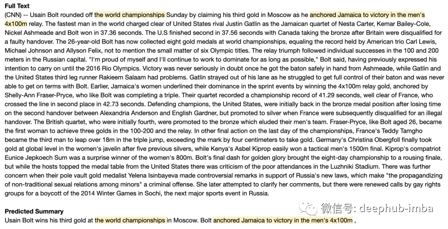
match = display_string_matching(dtf_test["text"][i], predicted[i], both=True, sentences=True, titles=["Full Text", "Predicted Summary"])

from IPython.core.display import display, HTML
display(HTML(match))

可以看到预测包含原始摘要中提到的大部分信息。 正如提取算法所期望的那样,预测的摘要完全包含在文本中:模型认为这 3 个句子是最重要的。 我们可以将此作为下面更为先进方法的基线。
Seq2Seq
序列到序列模型(2014)是一种神经网络的架构,它以来自一个域(即文本词汇表)的序列作为输入并输出另一个域(即摘要词汇表)中的新序列。 Seq2Seq 模型通常具有以下关键特征:
- 序列作为语料库:将文本填充成相同长度的序列以获得特征矩阵。
- 词嵌入机制:特征学习技术,将词汇表中的词映射到实数向量,这些向量是根据出现在另一个词之前或之后的每个词的概率分布计算得出的。
- 编码器-解码器结构:编码器处理输入序列并返回其自己的内部状态,作为解码器的上下文输入,解码器根据之前的词预测目标序列的下一个词。
- 训练模型和预测模型:训练中使用的模型不直接用于预测。事实上,会编写 2 个神经网络(都具有编码器-解码器结构),一个用于训练,另一个(称为“推理模型”)通过利用训练模型中的一些层来生成预测。
由于我们要将文本转换为单词序列,因此我们必须要对数据进行处理:
- 正确的序列大小,因为我们的语料库有不同的长度
- 我们的模型必须记住多少单词,并且排除稀有的单词
下面将清理和分析数据以解决这两个问题。
## create stopwords
lst_stopwords = nltk.corpus.stopwords.words("english")
## add words that are too frequent
lst_stopwords = lst_stopwords + ["cnn","say","said","new"]

## cleaning function
def utils_preprocess_text(txt, punkt=True, lower=True, slang=True, lst_stopwords=None, stemm=False, lemm=True):
    ### separate sentences with '. '
    txt = re.sub(r'\.(?=[^ \W\d])', '. ', str(txt))
    ### remove punctuations and characters
    txt = re.sub(r'[^\w\s]', '', txt) if punkt is True else txt
    ### strip
    txt = " ".join([word.strip() for word in txt.split()])
    ### lowercase
    txt = txt.lower() if lower is True else txt
    ### slang
    txt = contractions.fix(txt) if slang is True else txt
    ### tokenize (convert from string to list)
    lst_txt = txt.split()
    ### stemming (remove -ing, -ly, ...)
    if stemm is True:
        ps = nltk.stem.porter.PorterStemmer()
        lst_txt = [ps.stem(word) for word in lst_txt]
    ### lemmatization (convert the word into root word)
    if lemm is True:
        lem = nltk.stem.wordnet.WordNetLemmatizer()
        lst_txt = [lem.lemmatize(word) for word in lst_txt]
    ### remove Stopwords
    if lst_stopwords is not None:
        lst_txt = [word for word in lst_txt if word not in
                   lst_stopwords]
    ### back to string
    txt = " ".join(lst_txt)
    return txt

## apply function to both text and summaries
dtf_train["text_clean"] = dtf_train["text"].apply(lambda x: utils_preprocess_text(x, punkt=True, lower=True, slang=True, lst_stopwords=lst_stopwords, stemm=False, lemm=True))

dtf_train["y_clean"] = dtf_train["y"].apply(lambda x: utils_preprocess_text(x, punkt=True, lower=True, slang=True, lst_stopwords=lst_stopwords, stemm=False, lemm=True))
现在我们来看看长度分布:
## count
dtf_train['word_count'] = dtf_train[column].apply(lambda x: len(nltk.word_tokenize(str(x))) )

## plot
sns.distplot(dtf_train["word_count"], hist=True, kde=True, kde_kws={"shade":True})

X_len = 400
y_len = 40
我们来分析词频:
lst_tokens = nltk.tokenize.word_tokenize(dtf_train["text_clean"].str.cat(sep=" "))
ngrams = [1]

## calculate
dtf_freq = pd.DataFrame()
for n in ngrams:
   dic_words_freq = nltk.FreqDist(nltk.ngrams(lst_tokens, n))
   dtf_n = pd.DataFrame(dic_words_freq.most_common(), columns=
                        ["word","freq"])
   dtf_n["ngrams"] = n
   dtf_freq = dtf_freq.append(dtf_n)
   dtf_freq["word"] = dtf_freq["word"].apply(lambda x: "
                         ".join(string for string in x) )
   dtf_freq_X= dtf_freq.sort_values(["ngrams","freq"], ascending=
                         [True,False])

## plot
sns.barplot(x="freq", y="word", hue="ngrams", dodge=False,
 data=dtf_freq.groupby('ngrams')["ngrams","freq","word"].head(30))
plt.show()
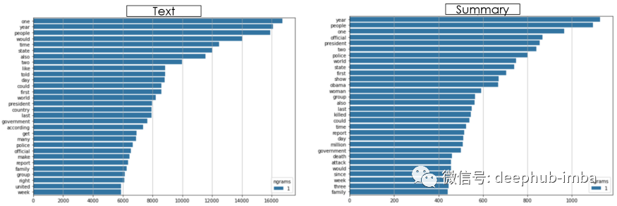
thres = 5 #<-- min frequency
X_top_words = len(dtf_freq_X[dtf_freq_X["freq"]>thres])
y_top_words = len(dtf_freq_y[dtf_freq_y["freq"]>thres])
这样就ok了,下面将通过使用 tensorflow/keras 将预处理的语料库转换为序列列表来创建特征矩阵:
lst_corpus = dtf_train["text_clean"]
## tokenize text
tokenizer = kprocessing.text.Tokenizer(num_words=X_top_words, lower=False, split=' ', oov_token=None,
filters='!"#$%&()*+,-./:;<=>?@[\\]^_`{|}~\t\n')
tokenizer.fit_on_texts(lst_corpus)
dic_vocabulary = {"<PAD>":0}
dic_vocabulary.update(tokenizer.word_index)
## create sequence
lst_text2seq= tokenizer.texts_to_sequences(lst_corpus)
## padding sequence
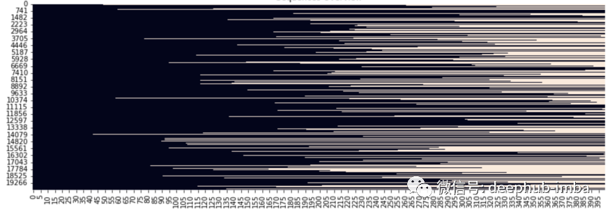
X_train = kprocessing.sequence.pad_sequences(lst_text2seq,
maxlen=15, padding="post", truncating="post")
特征矩阵 X_train 具有 N 个文档 x 序列最大长度的形状。 让我们可视化一下:
sns.heatmap(X_train==0, vmin=0, vmax=1, cbar=False)
plt.show()
除此以外,还需要对测试集进行相同的特征工程:
## text to sequence with the fitted tokenizer
lst_text2seq = tokenizer.texts_to_sequences(dtf_test["text_clean"])

## padding sequence
X_test = kprocessing.sequence.pad_sequences(lst_text2seq, maxlen=15,
             padding="post", truncating="post")
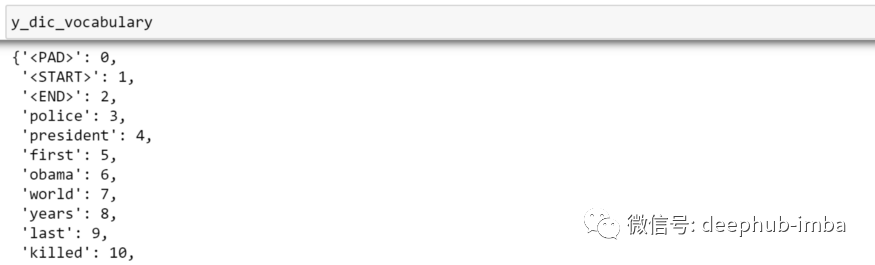
现在就可以处理摘要了。 在应用相同的特征工程策略之前,需要在每个摘要中添加两个特殊标记,以确定文本的开头和结尾。
# Add START and END tokens to the summaries (y)
special_tokens = ("<START>", "<END>")
dtf_train["y_clean"] = dtf_train['y_clean'].apply(lambda x:
                     special_tokens[0]+' '+x+' '+special_tokens[1])
dtf_test["y_clean"] = dtf_test['y_clean'].apply(lambda x:
                     special_tokens[0]+' '+x+' '+special_tokens[1])
# check example
dtf_test["y_clean"][i]

现在我们可以通过利用与以前相同的代码创建摘要的特征矩阵。预测时将使用开始标记开始预测,当结束标记出现时,预测文本将停止。
对于词嵌入这里有 2 个选项:从头开始训练我们的词嵌入模型或使用预训练的模型。 在 Python 中,可以 genism-data 加载预训练的 Word Embedding 模型:
import gensim_api
nlp = gensim_api.load("glove-wiki-gigaword-300")
这里推荐使用斯坦福的 GloVe,这是一种在 Wikipedia、Gigaword 和 Twitter 语料库上训练的无监督学习算法。 可以将任何单词转换为向量:
word = "home"
nlp[word].shape

>>> (300,)
这些词向量可以在神经网络中用作权重。 为了做到这一点,我们需要创建一个嵌入矩阵,以便 id N 的单词的向量位于第 N 行。
## start the matrix (length of vocabulary x vector size) with all 0s
X_embeddings = np.zeros((len(X_dic_vocabulary)+1, 300))for word,idx in X_dic_vocabulary.items():
    ## update the row with vector
    try:
        X_embeddings[idx] =  nlp[word]
    ## if word not in model then skip and the row stays all 0s
    except:
        pass
上面的代码生成从语料库中提取的词嵌入的矩阵。 语料库矩阵应会在编码器嵌入层中使用,而摘要矩阵会在解码器层中使用。 输入序列中的每个 id 都将用作访问嵌入矩阵的索引。 该嵌入层的输出将是一个 2D 矩阵,其中输入序列中的每个词 id 都有一个词向量(序列长度 x 向量大小):

下面就是构建编码器-解码器模型的时候了。 首先,我们需要确认正确的输入和输出:
输入是X(文本序列)加上y(摘要序列),并且需要隐藏摘要的最后一个单词
目标应该是没有开始标记的y(汇总序列)。
将输入文本提供给编码器以了解上下文,然后向解码器展示摘要如何开始,模型将会学习预测摘要如何结束。 这是一种称为“teacher forcing”的训练策略,它使用目标而不是网络生成的输出,以便它可以学习预测开始标记之后的单词,然后是下一个单词,依此类推。

本文将提出两个不同版本的 Seq2Seq,下面是我们使用的最简单的版本:
一个嵌入层,它将从头开始创建一个词嵌入。一个单向 LSTM 层,它返回一个序列以及单元状态和隐藏状态
最后一个Time Distributed Dense layer,它一次将相同的密集层(相同的权重)应用于 LSTM 输出,每次一个时间步长,这样输出层只需要一个与每个 LSTM 单元的连接。
lstm_units = 250
embeddings_size = 300

##------------ ENCODER (embedding + lstm) ------------------------##
x_in = layers.Input(name="x_in", shape=(X_train.shape[1],))

### embedding
layer_x_emb = layers.Embedding(name="x_emb",
                               input_dim=len(X_dic_vocabulary),
                               output_dim=embeddings_size,
                               trainable=True)
x_emb = layer_x_emb(x_in)

### lstm
layer_x_lstm = layers.LSTM(name="x_lstm", units=lstm_units,
                           dropout=0.4, return_sequences=True,
                           return_state=True)
x_out, state_h, state_c = layer_x_lstm(x_emb)

##------------ DECODER (embedding + lstm + dense) ----------------##
y_in = layers.Input(name="y_in", shape=(None,))

### embedding
layer_y_emb = layers.Embedding(name="y_emb",
                               input_dim=len(y_dic_vocabulary),
                               output_dim=embeddings_size,
                               trainable=True)
y_emb = layer_y_emb(y_in)

### lstm
layer_y_lstm = layers.LSTM(name="y_lstm", units=lstm_units,
                           dropout=0.4, return_sequences=True,
                           return_state=True)
y_out, _, _ = layer_y_lstm(y_emb, initial_state=[state_h, state_c])

### final dense layers
layer_dense = layers.TimeDistributed(name="dense",          layer=layers.Dense(units=len(y_dic_vocabulary), activation='softmax'))
y_out = layer_dense(y_out)

##---------------------------- COMPILE ---------------------------##
model = models.Model(inputs=[x_in, y_in], outputs=y_out,
                     name="Seq2Seq")
model.compile(optimizer='rmsprop',
              loss='sparse_categorical_crossentropy',
              metrics=['accuracy'])
model.summary()

如果你觉得上面的代码比较简单,以下是 Seq2Seq 算法的高级(并且非常重)版本:
嵌入层,利用 GloVe 的预训练权重。3 个双向 LSTM 层,在两个方向上处理序列。最后的Time Distributed Dense layer(与之前相同)
lstm_units = 250

##-------- ENCODER (pre-trained embeddings + 3 bi-lstm) ----------##
x_in = layers.Input(name="x_in", shape=(X_train.shape[1],))

### embedding
layer_x_emb = layers.Embedding(name="x_emb",
          input_dim=X_embeddings.shape[0],
          output_dim=X_embeddings.shape[1],
          weights=[X_embeddings], trainable=False)
x_emb = layer_x_emb(x_in)

### bi-lstm 1
layer_x_bilstm = layers.Bidirectional(layers.LSTM(units=lstm_units,
                 dropout=0.2, return_sequences=True,
                 return_state=True), name="x_lstm_1")
x_out, _, _, _, _ = layer_x_bilstm(x_emb)

### bi-lstm 2
layer_x_bilstm = layers.Bidirectional(layers.LSTM(units=lstm_units,
                 dropout=0.2, return_sequences=True,
                 return_state=True), name="x_lstm_2")
x_out, _, _, _, _ = layer_x_bilstm(x_out)

### bi-lstm 3 (here final states are collected)
layer_x_bilstm = layers.Bidirectional(layers.LSTM(units=lstm_units,
                 dropout=0.2, return_sequences=True,
                 return_state=True), name="x_lstm_3")
x_out, forward_h, forward_c, backward_h, backward_c = layer_x_bilstm(x_out)
state_h = layers.Concatenate()([forward_h, backward_h])
state_c = layers.Concatenate()([forward_c, backward_c])

##------ DECODER (pre-trained embeddings + lstm + dense) ---------##
y_in = layers.Input(name="y_in", shape=(None,))

### embedding
layer_y_emb = layers.Embedding(name="y_emb",
               input_dim=y_embeddings.shape[0],
               output_dim=y_embeddings.shape[1],
               weights=[y_embeddings], trainable=False)
y_emb = layer_y_emb(y_in)

### lstm
layer_y_lstm = layers.LSTM(name="y_lstm", units=lstm_units*2, dropout=0.2, return_sequences=True, return_state=True)
y_out, _, _ = layer_y_lstm(y_emb, initial_state=[state_h, state_c])

### final dense layers
layer_dense = layers.TimeDistributed(name="dense",
              layer=layers.Dense(units=len(y_dic_vocabulary),
               activation='softmax'))
y_out = layer_dense(y_out)

##---------------------- COMPILE ---------------------------------##
model = models.Model(inputs=[x_in, y_in], outputs=y_out,
                     name="Seq2Seq")
model.compile(optimizer='rmsprop',
              loss='sparse_categorical_crossentropy',
              metrics=['accuracy'])
model.summary()
下面就可以实际进行训练了,在实际测试集上进行测试之前,我将保留一小部分训练集进行验证。
## train
training = model.fit(x=[X_train, y_train[:,:-1]],
                     y=y_train.reshape(y_train.shape[0],
                                       y_train.shape[1],
                                       1)[:,1:],
                     batch_size=128,
                     epochs=100,
                     shuffle=True,
                     verbose=1,
                     validation_split=0.3,
                     callbacks=[callbacks.EarlyStopping(
                                monitor='val_loss',
                                mode='min', verbose=1, patience=2)]
                      )
## plot loss and accuracy
metrics = [k for k in training.history.keys() if ("loss" not in k) and ("val" not in k)]
fig, ax = plt.subplots(nrows=1, ncols=2, sharey=True)

ax[0].set(title="Training")
ax11 = ax[0].twinx()
ax[0].plot(training.history['loss'], color='black')
ax[0].set_xlabel('Epochs')
ax[0].set_ylabel('Loss', color='black')
for metric in metrics:
    ax11.plot(training.history[metric], label=metric)
ax11.set_ylabel("Score", color='steelblue')
ax11.legend()

ax[1].set(title="Validation")
ax22 = ax[1].twinx()
ax[1].plot(training.history['val_loss'], color='black')
ax[1].set_xlabel('Epochs')
ax[1].set_ylabel('Loss', color='black')
for metric in metrics:
     ax22.plot(training.history['val_'+metric], label=metric)
ax22.set_ylabel("Score", color="steelblue")
plt.show()
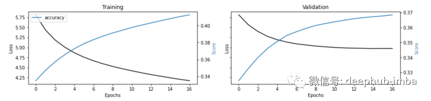
这里在回调中使用了 EarlyStopping,当监控的指标(即验证损失)停止改进时应该停止训练。 这对于节省时间特别有用,尤其是对于像这样的长时间的训练。 在不利用 GPU 的情况下运行 Seq2Seq 算法非常困难,因为同时训练了 2 个模型(编码器-解码器)所以GPU是必须的。
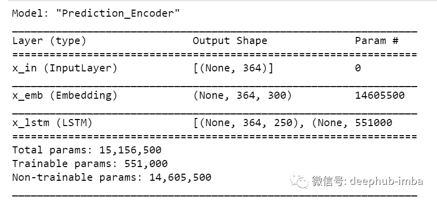
训练结束了,但是工作还没结束! 作为测试 Seq2Seq 模型的最后一步,需要构建推理模型来生成预测。 预测编码器将一个新序列(X_test)作为输入,并返回最后一个 LSTM 层的输出及其状态。
# Prediction Encoder
encoder_model = models.Model(inputs=x_in, outputs=[x_out, state_h, state_c], name="Prediction_Encoder")
encoder_model.summary()
另一方面,预测解码器将起始标记、编码器的输出及其状态作为输入,并返回新状态以及词汇表上的概率分布(概率最高的词将是预测) .
## double the lstm units if you used bidirectional lstm
lstm_units = lstm_units*2 if any("Bidirectional" in str(layer) for layer in model.layers) else lstm_units

## states of the previous time step
encoder_out = layers.Input(shape=(X_train.shape[1], lstm_units))
state_h, state_c = layers.Input(shape=(lstm_units,)), layers.Input(shape=(lstm_units,))

## decoder embeddings
y_emb2 = layer_y_emb(y_in)

## lstm to predict the next word
y_out2, state_h2, state_c2 = layer_y_lstm(y_emb2, initial_state=[state_h, state_c])

## softmax to generate probability distribution over the vocabulary
probs = layer_dense(y_out2)

## compile
decoder_model = models.Model(inputs=[y_in, encoder_out, state_h, state_c], outputs=[probs, state_h2, state_c2], name="Prediction_Decoder")

decoder_model.summary()
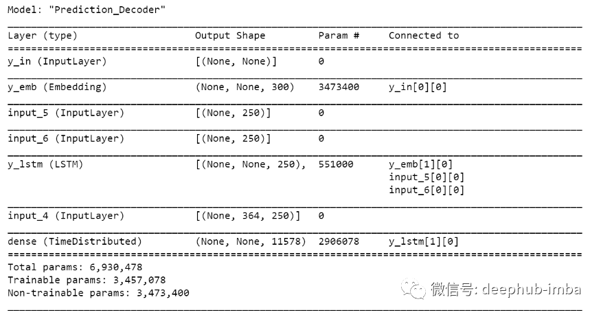
在使用起始标记和编码器状态进行第一次预测后,解码器使用生成的词和新状态来预测新词和新状态。 该迭代将继续进行,直到模型最终预测到结束标记或预测的摘要达到其最大长度。
下面就上述循环来生成预测并测试 Seq2Seq 模型的代码:
# Predict
max_seq_lenght = X_test.shape[1]
predicted = []
for x in X_test:
   x = x.reshape(1,-1)
   ## encode X
   encoder_out, state_h, state_c = encoder_model.predict(x)
   ## prepare loop
   y_in = np.array([fitted_tokenizer.word_index[special_tokens[0]]])
   predicted_text = ""
   stop = False
   while not stop:
   ## predict dictionary probability distribution
        probs, new_state_h, new_state_c = decoder_model.predict(
                          [y_in, encoder_out, state_h, state_c])

        ## get predicted word
        voc_idx = np.argmax(probs[0,-1,:])
        pred_word = fitted_tokenizer.index_word[voc_idx]

        ## check stop
        if (pred_word != special_tokens[1]) and
           (len(predicted_text.split()) < max_seq_lenght):
            predicted_text = predicted_text +" "+ pred_word
        else:
            stop = True

        ## next
        y_in = np.array([voc_idx])
        state_h, state_c = new_state_h, new_state_c

   predicted_text = predicted_text.replace(
                    special_tokens[0],"").strip()
   predicted.append(predicted_text)

该模型理解上下文和关键信息,但它对词汇的预测很差。 发生这种情况是因为我在这个实验的完整数据集的一小部分上运行了 Seq2Seq “简化版”。 如果像改进的话可以添加更多数据并提高性能。
Transformers
Transformers 是 Google 的论文 Attention is All You Need (2017) 提出的一种新的建模技术,其中证明序列模型(如 LSTM)可以完全被注意力机制取代,甚至可以获得更好的性能。 这些语言模型可以通过一次处理所有序列并映射单词之间的依赖关系来执行任何 NLP 任务,无论它们在文本中相距多远。在他们的词嵌入中,同一个词可以根据上下文有不同的向量。 最著名的语言模型是 Google 的 BERT 和 OpenAI 的 GPT。
Facebook 的 BART(双向自回归Transformers)使用标准的 Seq2Seq 双向编码器(如 BERT)和从左到右的自回归解码器(如 GPT)。 可以说:BART = BERT + GPT。
Transformers 模型的主要库是 HuggingFace 的Transformer:
def bart(corpus, max_len):
    nlp = transformers.pipeline("summarization")
    lst_summaries = [nlp(txt,
                         max_length=max_len
                         )[0]["summary_text"].replace(" .", ".")
                     for txt in corpus]
    return lst_summaries
## Apply the function to corpus
predicted = bart(corpus=dtf_test["text"], max_len=y_len)

预测简短而且有效。 对于大多数 NLP 任务,Transformer 模型似乎是表现最好的。并且对于一般的使用,完全可以使用HuggingFace 的与训练模型,可以提高不少效率
总结
本文演示了如何将不同的 NLP 模型应用于文本摘要用例。 这里比较了 3 种流行的方法:无监督 TextRank、两个不同版本的基于词嵌入的监督 Seq2Seq 和预训练 BART。并且还包含了特征工程、模型设计、评估和可视化。
以下是本文的完整代码:
数据集:
https://huggingface.co/datasets/cnn_dailymail
作者:Mauro Di Pietro