
Keras
Keras 的核心数据结构是 model,一种组织网络层的方式。最简单的模型是 Sequential 顺序模型,它由多个网络层线性堆叠。对于更复杂的结构,你应该使用 Keras 函数式 API,它允许构建任意的神经网络图。
练习一 线性回归
导入包
import keras
import numpy as np
import matplotlib.pyplot as plt
#按顺序构成的模型
from keras.models import Sequential
#Dense全连接层
from keras.layers import Dense
构造数据
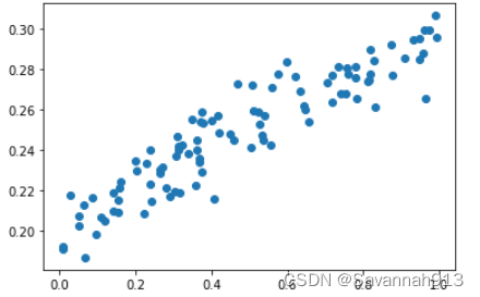
#使用numpy生成100个随机点
x_data = np.random.rand(100)
#噪音(扰动)
noise = np.random.normal(0,0.01,x_data.shape)
#0.1相当于斜率,0.2相当于截距
y_data = x_data*0.1 + 0.2 + noise #加上噪声的扰动更符合真实情况
#显示随机点
plt.scatter(x_data,y_data)
plt.show()
numpy.random.normal
numpy.random.normal(loc=0.0, scale=1.0, size=None)
loc:均值,scale:标准差。(正态分布)
建立网络模型
#构建一个顺序模型
model = Sequential()
#光标放在参数上,shift+Tab键查看参数的详细解释
#units表示输出参数的维度,input_dim表示输入参数的维度
model.add(Dense(units=1,input_dim=1))
#编译这个模型
model.compile(optimizer="sgd",loss="mse")
使用 Sequential() 搭建模型
引用(5条消息) keras创建model的两种方式_tjj1057813680的博客-CSDN博客_keras model.add
Sequential是实现全连接网络的最好方式, 是多个网络层的线性堆栈。**model = Sequential()**创建一个线性模型后,可以用add()将不同层网络叠加,构成一个网络
from keras.layers import Dense,Activation

model.add(Dense(units=64,input_dim=100))
model.add(Activation('relu'))
model.add(Dense(units=10))
model.add(Activation('softmax'))
或者是直接输入一个list来完成Sequential模型的创建
model = Sequential([
                  (Dense(units=64,input_dim=100)),
                  (Activation('relu')),
                  (Dense(units=10)),
                  (Activation('softmax'))
                  ])
Dense就是常用的全连接层
Dense(units, activation=None, use_bias=True, kernel_initializer='glorot_uniform', bias_initializer='zeros', kernel_regularizer=None, bias_regularizer=None, activity_regularizer=None, kernel_constraint=None, bias_constraint=None)
units:正整数,输出空间维度
activation:激活函数
kernel_initializer:
kernel
权值矩阵的初始化器 (详见 initializers)。
bias_initializer: 偏置向量的初始化器 (see initializers).
regularizer:正则化函数
constraints:约束函数
compile参数介绍
model.compile(
   optimizer,
   loss = None,
   metrics = None
)
常用的三个参数
optimizer:优化器,用于控制梯度裁剪。必选项
**sgd**:随机梯度下降优化器
loss:损失函数(或称目标函数、优化评分函数)。必选项
**mse**:mean_squared_error,均方误差
metrics:评价函数用于评估当前训练模型的性能。当模型编译后(compile),评价函数应该作为 metrics 的参数来输入。评价函数和损失函数相似,只不过评价函数的结果不会用于训练过程中。
原文链接:https://blog.csdn.net/huang1024rui/article/details/120055487
训练模型(不断迭代)
模型的训练中一次训练一个批次,几十个不等
#训练3001个批次
for step in range(3001):
    #每次训练一个批次
    cost = model.train_on_batch(x_data,y_data)
    #500个batch打印一次cost值
    if step % 500 == 0:
        print("cost:",cost)

#打印权值和偏置值
w,b = model.layers[0].get_weights()
print("w:",w,"b:",b)
#此处layers[0]因为只构建了一层网络

#x_data输入网络中,得到预测值y_pred
y_pred = model.predict(x_data)

#显示随机点
plt.scatter(x_data,y_data)
#显示预测结果
plt.plot(x_data,y_pred,"r-",lw=3)
plt.show()
train_on_batch函数训练数据
model.train_on_batch(x_data,y_data)接受单批数据,执行反向传播,然后更新模型参数,数据的批量大小可以使任意的,属于精细化控制训练模型,但是通常我们不要求特别精细,一般使用fit_generator训练方式。
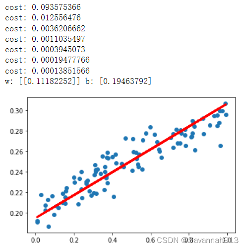
由上图观察得,打印出来的cost值越来越小,训练出最终的参数w,b,以及最终拟合出来的红色直线,这里的w,b就是直线的斜率和截距,在最开始生成数据时,用的斜率和截距分别是0.1和0.2,显然,经过训练后,w和b已经很接近这两个值了,但是由于noise的作用,以及训练次数有限的原因,并不会完全相等。
线性回归练习的完整代码
import keras
import numpy as np
import matplotlib.pyplot as plt
#按顺序构成的模型
from keras.models import Sequential
#Dense全连接层
from keras.layers import Dense

#使用numpy生成100个随机点
x_data = np.random.rand(100)
#噪音(扰动)
noise = np.random.normal(0,0.01,x_data.shape)
#0.1相当于斜率,0.2相当于截距
y_data = x_data*0.1 + 0.2 + noise #加上噪声的扰动更符合真实情况
#显示随机点
plt.scatter(x_data,y_data)
plt.show()

#构建一个顺序模型
model = Sequential()
#光标放在参数上,shift+Tab键查看参数的详细解释
#units表示输出参数的维度,input_dim表示输入参数的维度
model.add(Dense(units=1,input_dim=1))
#编译这个模型
model.compile(optimizer="sgd",loss="mse")

#训练3001个批次
for step in range(3001):
    #每次训练一个批次
    cost = model.train_on_batch(x_data,y_data)
    #500个batch打印一次cost值
    if step % 500 == 0:
        print("cost:",cost)

#打印权值和偏置值
w,b = model.layers[0].get_weights()
print("w:",w,"b:",b)
#此处layers[0]因为只构建了一层网络

#x_data输入网络中,得到预测值y_pred
y_pred = model.predict(x_data)

#显示随机点
plt.scatter(x_data,y_data)
#显示预测结果
plt.plot(x_data,y_pred,"r-",lw=3)
plt.show()
练习二 非线性回归
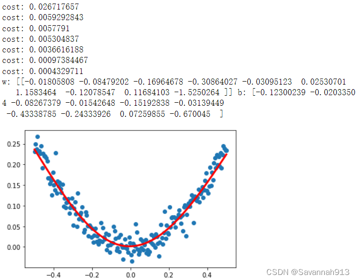
非线性回归和线性回归的最大区别在于是否有激活函数,如果没有激活函数,那么这个网络只能表现出线性回归的形式,对于非线性分布并不能很好地拟合。
激活函数
常用的激活函数有:sigmoid函数,tanh函数,Relu函数,Leaky Relu函数
详解激活函数(Sigmoid/Tanh/ReLU/Leaky ReLu等) - 知乎 (zhihu.com)
构造数据
import keras
import numpy as np
import matplotlib.pyplot as plt
#按顺序构成的模型
from keras.models import Sequential
#导入学习率大于sgd的优化器
from keras.optimizers import SGD
#Dense全连接层,激活函数
from keras.layers import Dense,Activation
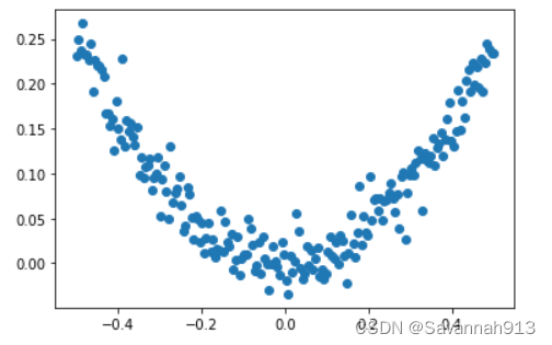
#生成数据,在-0.5和0.5之间生成200个点
x_data = np.linspace(-0.5,0.5,200)
#生成噪声
noise = np.random.normal(0,0.02,x_data.shape)
y_data = np.square(x_data)+noise
#显示随机点
plt.scatter(x_data,y_data)
plt.show()
构建网络模型
model = Sequential()
#units表示输出参数的维度,input_dim表示输入参数的维度
#由于上述数据,输入和输出都是一维的(一个x,一个y)那么,
#可以采用增加隐藏层的方式进行拟合1—10—1
#对于非线性回归,必须加入激活函数,没有激活函数,他表现为线性回归
#每层都要加上一个激活函数
model.add(Dense(units=10,input_dim=1))#隐藏层(输出层10个单元)
model.add(Activation("tanh"))
#加激活函数的其他方法:
#model.add(Dense(units=10,input_dim=1,activation="Relu"))
model.add(Dense(units=1))#输出层的输入时隐藏层的输出,可以不具体指定
model.add(Activation("tanh"))
#导入学习率高一些的sgd优化器,定义优化算法
#学习率太低的话,迭代次数的要求就会很高
sgd = SGD(lr=0.3)
#编译这个模型,mse:均方误差
model.compile(optimizer=sgd,loss="mse")
进行训练并显示预测结果
#训练3001个批次
for step in range(3001):
    #每次训练一个批次
    cost = model.train_on_batch(x_data,y_data)
    #500个batch打印一次cost值
    if step % 500 == 0:
        print("cost:",cost)

#打印权值和偏置值
w,b = model.layers[0].get_weights()
print("w:",w,"b:",b)
#此处layers[0]因为只构建了一层网络

#x_data输入网络中,得到预测值y_pred
y_pred = model.predict(x_data)

#显示随机点
plt.scatter(x_data,y_data)
#显示预测结果
plt.plot(x_data,y_pred,"r-",lw=3)
plt.show()
练习三 MINI分类程序
导入包
#MNIST数据集是由0到9的数字图像构成的。训练图像有6万张,测试图像有1万张。
import numpy as np
#导入数据集
from keras.datasets import mnist
#导入工具包
from keras.utils import np_utils
from keras.models import Sequential
from keras.layers import Dense
from keras.optimizers import SGD
载入数据
#载入数据(训练集图像,训练集标签)(测试集图像,测试集标签)
(x_train,y_train),(x_test,y_test) = mnist.load_data()
print(x_train.shape)
print(y_train.shape)

调整数据
#将训练集和测试集图像数据维度进行调整,并进行归一化
#列数写成-1是让其生成一个合适的列数,此处生成的列数是28*28得到的
#imshow显示uint8型时是0~255范围,归一化会将图像矩阵转化到0-1之间
x_train = x_train.reshape(x_train.shape[0],-1)/255.0
x_test = x_test.reshape(x_test.shape[0],-1)/255.0
print(x_train.shape)
print(x_test.shape)
#转换成one-hot格式,分成10类
y_train = np_utils.to_categorical(y_train,num_classes=10)
y_test = np_utils.to_categorical(y_test,num_classes=10)
print(y_train)
print(y_test)

one-hot转换
** keras中多分类标签转换成One-hot**
链接:TensorFlow 中one_hot讲解以及多分类 标签与one-hot转换 - 掘金 (juejin.cn)
来源:稀土掘金
import numpy as np
from keras.utils import to_categorical

data = [1, 2, 3, 4, 5, 6, 7, 8, 9, 7]
data = array(data)
print(data)
# [1 2 3 4 5 6 7 8 9 7]

#有普通np数组转换为one-hot
one_hots = to_categorical(data)
print(one_hots)
# [[ 0.  1.  0.  0.  0.  0.  0.  0.  0.  0.]
#  [ 0.  0.  1.  0.  0.  0.  0.  0.  0.  0.]
#  [ 0.  0.  0.  1.  0.  0.  0.  0.  0.  0.]
#  [ 0.  0.  0.  0.  1.  0.  0.  0.  0.  0.]
#  [ 0.  0.  0.  0.  0.  1.  0.  0.  0.  0.]
#  [ 0.  0.  0.  0.  0.  0.  1.  0.  0.  0.]
#  [ 0.  0.  0.  0.  0.  0.  0.  1.  0.  0.]
#  [ 0.  0.  0.  0.  0.  0.  0.  0.  1.  0.]
#  [ 0.  0.  0.  0.  0.  0.  0.  0.  0.  1.]
#  [ 0.  0.  0.  0.  0.  0.  0.  1.  0.  0.]]

# 由one-hot转换为普通np数组
data = [argmax(one_hot)for one_hot in one_hots]
print(data)
# [1, 2, 3, 4, 5, 6, 7, 8, 9, 7]
创建模型
#创建模型,输入784个神经元,输出10个神经元
model = Sequential([
    #偏置值默认初始化为zero,此处设置为one
    Dense(units=10,input_dim=784,bias_initializer="one",activation="softmax")
])

#定义优化器
sgd = SGD(lr=0.2)

#编译模型,定义损失函数,metrics训练过程中计算准确率
model.compile(
    optimizer = sgd,
    loss = "mse",
    metrics = ["accuracy"],
)
print(y_train.shape,x_train.shape)
#(60000, 10, 10, 10) (60000, 784)
构建神经网络,输入维度784(列),输出维度units为10,偏差初始化1,激活函数采用softmax,优化器采用sgd,loss采用 均方误差进行计算,训练过程中计算准确率用来评估模型。
训练数据
此处采用model.fit(x_train,y_train,batchsize=32,epochs=10)的方式进行数据的训练,这种方式是一次把训练数据全部加载到内存中,每次批处理batch_size个数据来更新模型参数,eg:总数据量有6000,每批次处理的数据量是32,那么需要处理6000/32批次,而epochs等于10表示周期,即总共需要处理6000/32*10批次。所有训练集重复训练10次。
#训练模型-----.fit训练数据
model.fit(x_train,y_train,batch_size=32,epochs=10)

#评估模型
loss,accuracy = model.evaluate(x_test,y_test)

print("test loss",loss)
print("accuracy",accuracy)
完整代码
#MNIST数据集是由0到9的数字图像构成的。训练图像有6万张,测试图像有1万张。
import numpy as np
#导入数据集
from keras.datasets import mnist
#导入工具包
from keras.utils import np_utils
from keras.models import Sequential
from keras.layers import Dense
from keras.optimizers import SGD

#载入数据(训练集图像,训练集标签)(测试集图像,测试集标签)
(x_train,y_train),(x_test,y_test) = mnist.load_data()
print(x_train.shape)
print(y_train.shape)

#将训练集和测试集图像数据维度进行调整,并进行归一化
#列数写成-1是让其生成一个合适的列数,此处生成的列数是28*28得到的
#imshow显示uint8型时是0~255范围,归一化会将图像矩阵转化到0-1之间
x_train = x_train.reshape(x_train.shape[0],-1)/255.0#(60000, 784)
x_test = x_test.reshape(x_test.shape[0],-1)/255.0#(10000, 784)

#转换成one-hot格式,分成10类
y_train = np_utils.to_categorical(y_train,num_classes=10)
y_test = np_utils.to_categorical(y_test,num_classes=10)

#创建模型,输入784个神经元,输出10个神经元
model = Sequential([
    #偏置值默认初始化为zero,此处设置为one
    Dense(units=10,input_dim=784,bias_initializer="one",activation="softmax")
])

#定义优化器
sgd = SGD(lr=0.2)

#编译模型,定义损失函数,metrics训练过程中计算准确率
model.compile(
    optimizer = sgd,
    loss = "mse",
    metrics = ["accuracy"],
)
print(y_train.shape,x_train.shape)
#(60000, 10, 10, 10) (60000, 784)

#训练模型-----.fit训练数据
model.fit(x_train,y_train,batch_size=32,epochs=10)

#评估模型
loss,accuracy = model.evaluate(x_test,y_test)

print("test loss",loss)
print("accuracy",accuracy)
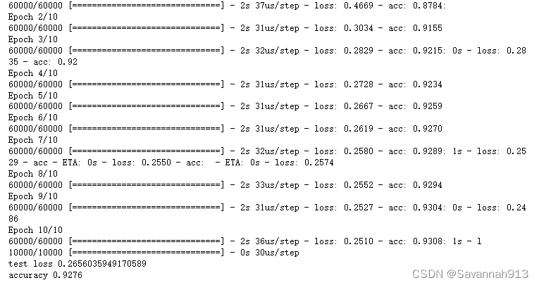
运行截图
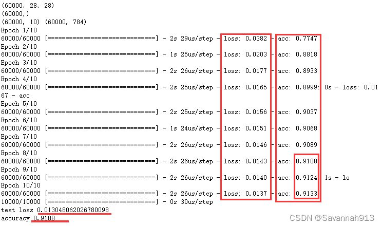
由运行结果可知,通过对模型不断训练,误差会越来越小,精确率越来越高,当到一定程度后,精确度会处于基本饱和。
交叉熵
在上一部分的代码中,编译模型的过程如下所示,采用均方差mse的方式作为loss function,我们也可以采用交叉熵作为loss function,而且使用交叉熵来训练数据会使得精确率收敛得更快一些。
#编译模型,定义损失函数,metrics训练过程中计算准确率
model.compile(
    optimizer = sgd,
    loss = "mse",#使用均方差作为损失函数
    metrics = ["accuracy"],
)
将损失函数换成交叉熵只需要改变参数loss的值即可
#编译模型,定义损失函数,metrics训练过程中计算准确率
model.compile(
    optimizer = sgd,
    loss = "categorical_crossentropy",#采用交叉熵作为损失函数
    metrics = ["accuracy"],
)
观察均方差和交叉熵的准确率变化
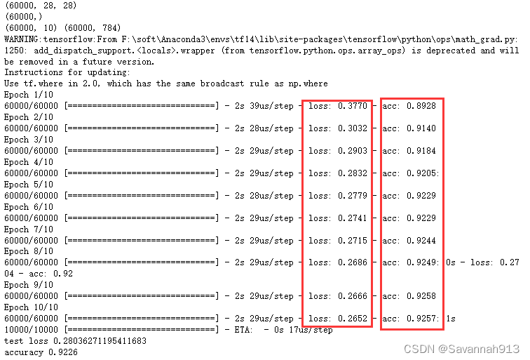
显然使用均方差在第10个周期时准确率也没有高于92%,但是使用交叉熵在第4个周期就高于92%。所以交叉熵的准确率更高一些。
正则化
Dropout应用
建立**两层隐藏层**来训练同样数据量的数据
#Dropout
#MNIST数据集是由0到9的数字图像构成的。训练图像有6万张,测试图像有1万张。
import numpy as np
#导入数据集
from keras.datasets import mnist
#导入工具包
from keras.utils import np_utils
from keras.models import Sequential
from keras.layers import Dense
from keras.optimizers import SGD

import warnings
warnings.filterwarnings("ignore")

#载入数据(训练集图像,训练集标签)(测试集图像,测试集标签)
(x_train,y_train),(x_test,y_test) = mnist.load_data()
print(x_train.shape)
print(y_train.shape)

#将训练集和测试集图像数据维度进行调整,并进行归一化
#列数写成-1是让其生成一个合适的列数,此处生成的列数是28*28得到的
#imshow显示uint8型时是0~255范围,归一化会将图像矩阵转化到0-1之间
x_train = x_train.reshape(x_train.shape[0],-1)/255.0#(60000, 784)
x_test = x_test.reshape(x_test.shape[0],-1)/255.0#(10000, 784)

#转换成one-hot格式,分成10类
y_train = np_utils.to_categorical(y_train,num_classes=10)
y_test = np_utils.to_categorical(y_test,num_classes=10)

#创建模型,输入784个神经元,输出10个神经元,添加隐藏层
model = Sequential([
    #偏置值默认初始化为zero,此处设置为one
    #只有第一层需要设置输入维度,第二次输入开始,不用设置输入维度,输入维度就是上一层输出的维度
    Dense(units=200,input_dim=784,bias_initializer="one",activation="tanh"),#隐藏层
    Dense(units=100,bias_initializer="one",activation="tanh"),#隐藏层
    Dense(units=10,bias_initializer="one",activation="softmax"),#输出层
])
#也可以在定义模型之后添加隐藏层
#model.add(Dense(...))
#定义优化器
sgd = SGD(lr=0.2)

#编译模型,定义损失函数,metrics训练过程中计算准确率
model.compile(
    optimizer = sgd,
    loss = "categorical_crossentropy",#采用交叉熵作为损失函数
    metrics = ["accuracy"],
)
print(y_train.shape,x_train.shape)
#(60000, 10, 10, 10) (60000, 784)

#训练模型-----.fit训练数据
model.fit(x_train,y_train,batch_size=32,epochs=10)

#评估训练集
loss,accuracy = model.evaluate(x_test,y_test)

print("\ntrain loss",loss)
print("accuracy",accuracy)

#评估测试集
loss,accuracy = model.evaluate(x_test,y_test)

print("test loss",loss)
print("accuracy",accuracy)
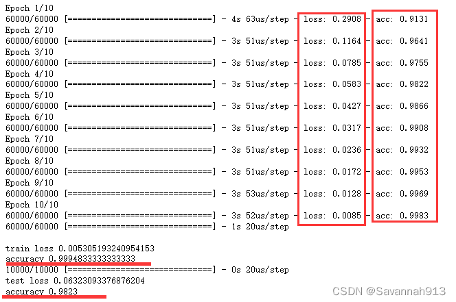
     显然增加了网络复杂程度之后对数据训练的准确度有大幅度提高,由之前的92%左右,到达98%左右。

    过拟合是一种训练集准确度很高,测试集准确度很低,即二者差距很大的情况,对于过拟合现象可以采用正则化的方法进行优化,eg:dropout随机失活正则化

    使用正则化方法在一定程度上可以减小训练集和测试集结果的差距,但是可会增大偏差
Dropout的使用方法就是在创建模型时增加一条
model.add(Dropout(rate=0.2, input_shape=(4,)))
导入Dropout的方法from keras.layers import Dropout
#创建模型,输入784个神经元,输出10个神经元,添加隐藏层
model = Sequential([
    #偏置值默认初始化为zero,此处设置为one
    #只有第一层需要设置输入维度,第二次输入开始,不用设置输入维度,输入维度就是上一层输出的维度
    Dense(units=200,input_dim=784,bias_initializer="one",activation="tanh"),#隐藏层
    #增加Dropout
    Dropout(0.4),#让该层40%的神经元不工作
    Dense(units=100,bias_initializer="one",activation="tanh"),#隐藏层
    Dropout(0.4),#让该层40%的神经元不工作
    Dense(units=10,bias_initializer="one",activation="softmax"),#输出层
])
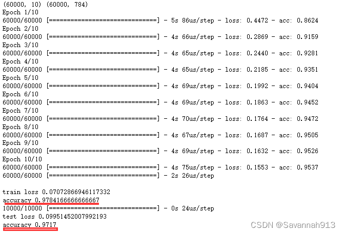
由该运行结果可以观察到,准确率整体降低,但是训练集和测试集的准确率差距变小了。
l2正则化应用
使用方法是在创建模型时,加上参数,kernel_regularizer=l2(0.0003)
Dense(units=200,input_dim=784,bias_initializer="one",activation="tanh",kernel_regularizer=l2(0.0003))
导入:from keras.regularizers import l2
#Dropout
#MNIST数据集是由0到9的数字图像构成的。训练图像有6万张,测试图像有1万张。
import numpy as np
#导入数据集
from keras.datasets import mnist
#导入工具包
from keras.utils import np_utils
from keras.models import Sequential
from keras.layers import Dense
from keras.layers import Dropout
from keras.optimizers import SGD
#正则化
from keras.regularizers import l2

import warnings
warnings.filterwarnings("ignore")

#载入数据(训练集图像,训练集标签)(测试集图像,测试集标签)
(x_train,y_train),(x_test,y_test) = mnist.load_data()
#print(x_train.shape)(60000, 28, 28)
#print(y_train.shape)

#将训练集和测试集图像数据维度进行调整,并进行归一化
#列数写成-1是让其生成一个合适的列数,此处生成的列数是28*28得到的
#imshow显示uint8型时是0~255范围,归一化会将图像矩阵转化到0-1之间
x_train = x_train.reshape(x_train.shape[0],-1)/255.0#(60000, 784)
x_test = x_test.reshape(x_test.shape[0],-1)/255.0#(10000, 784)

#转换成one-hot格式,分成10类
y_train = np_utils.to_categorical(y_train,num_classes=10)
y_test = np_utils.to_categorical(y_test,num_classes=10)

#创建模型,输入784个神经元,输出10个神经元,添加隐藏层
model = Sequential([
    #偏置值默认初始化为zero,此处设置为one
    #只有第一层需要设置输入维度,第二次输入开始,不用设置输入维度,输入维度就是上一层输出的维度
    Dense(units=200,input_dim=784,bias_initializer="one",activation="tanh",kernel_regularizer=l2(0.0003)),#隐藏层
    Dense(units=100,bias_initializer="one",activation="tanh",kernel_regularizer=l2(0.0003)),#隐藏层
    Dense(units=10,bias_initializer="one",activation="softmax",kernel_regularizer=l2(0.0003)),#输出层
])
#也可以在定义模型之后添加隐藏层
#model.add(Dense(...))
#定义优化器
sgd = SGD(lr=0.2)

#编译模型,定义损失函数,metrics训练过程中计算准确率
model.compile(
    optimizer = sgd,
    loss = "categorical_crossentropy",#采用交叉熵作为损失函数
    metrics = ["accuracy"],
)
print(y_train.shape,x_train.shape)
#(60000, 10, 10, 10) (60000, 784)

#训练模型-----.fit训练数据
model.fit(x_train,y_train,batch_size=32,epochs=10)

#评估训练集
loss,accuracy = model.evaluate(x_train,y_train)

print("\ntrain loss",loss)
print("accuracy",accuracy)

#评估测试集
loss,accuracy = model.evaluate(x_test,y_test)

print("test loss",loss)
print("accuracy",accuracy)

显然,这个运行结果和Dropout正则化差不多
优化器
#定义优化器
from keras.optimizers import SGD,Adam
sgd = SGD(lr=0.2)#学习率
adam = Adam(lr=0.001)#学习率
这两种优化器相对来说,Adam更优秀一些,Adam进行模型优化的速度比较快。
sdg优化器
#优化器
#MNIST数据集是由0到9的数字图像构成的。训练图像有6万张,测试图像有1万张。
import numpy as np
#导入数据集
from keras.datasets import mnist
#导入工具包
from keras.utils import np_utils
from keras.models import Sequential
from keras.layers import Dense
from keras.optimizers import SGD

import warnings
warnings.filterwarnings("ignore")

#载入数据(训练集图像,训练集标签)(测试集图像,测试集标签)
(x_train,y_train),(x_test,y_test) = mnist.load_data()

#将训练集和测试集图像数据维度进行调整,并进行归一化
#列数写成-1是让其生成一个合适的列数,此处生成的列数是28*28得到的
#imshow显示uint8型时是0~255范围,归一化会将图像矩阵转化到0-1之间
x_train = x_train.reshape(x_train.shape[0],-1)/255.0#(60000, 784)
x_test = x_test.reshape(x_test.shape[0],-1)/255.0#(10000, 784)

#转换成one-hot格式,分成10类
y_train = np_utils.to_categorical(y_train,num_classes=10)
y_test = np_utils.to_categorical(y_test,num_classes=10)

#创建模型,输入784个神经元,输出10个神经元
model = Sequential([
    #偏置值默认初始化为zero,此处设置为one
    Dense(units=10,input_dim=784,bias_initializer="one",activation="softmax")
])

#定义优化器
sgd = SGD(lr=0.2)#学习率

#编译模型,定义损失函数,metrics训练过程中计算准确率
model.compile(
    optimizer = sgd,
    loss = "categorical_crossentropy",#采用交叉熵作为损失函数
    metrics = ["accuracy"],
)
print(y_train.shape,x_train.shape)
#(60000, 10, 10, 10) (60000, 784)

#训练模型-----.fit训练数据
model.fit(x_train,y_train,batch_size=32,epochs=10)

#评估模型
loss,accuracy = model.evaluate(x_test,y_test)

print("test loss",loss)
print("accuracy",accuracy)

这是sgd的优化结果,才92.233%
采用Adam:
#优化器
#MNIST数据集是由0到9的数字图像构成的。训练图像有6万张,测试图像有1万张。
import numpy as np
#导入数据集
from keras.datasets import mnist
#导入工具包
from keras.utils import np_utils
from keras.models import Sequential
from keras.layers import Dense
from keras.optimizers import SGD,Adam

import warnings
warnings.filterwarnings("ignore")

#载入数据(训练集图像,训练集标签)(测试集图像,测试集标签)
(x_train,y_train),(x_test,y_test) = mnist.load_data()

#将训练集和测试集图像数据维度进行调整,并进行归一化
#列数写成-1是让其生成一个合适的列数,此处生成的列数是28*28得到的
#imshow显示uint8型时是0~255范围,归一化会将图像矩阵转化到0-1之间
x_train = x_train.reshape(x_train.shape[0],-1)/255.0#(60000, 784)
x_test = x_test.reshape(x_test.shape[0],-1)/255.0#(10000, 784)

#转换成one-hot格式,分成10类
y_train = np_utils.to_categorical(y_train,num_classes=10)
y_test = np_utils.to_categorical(y_test,num_classes=10)

#创建模型,输入784个神经元,输出10个神经元
model = Sequential([
    #偏置值默认初始化为zero,此处设置为one
    Dense(units=10,input_dim=784,bias_initializer="one",activation="softmax")
])

#定义优化器
sgd = SGD(lr=0.2)#学习率
adam = Adam(lr=0.001)#学习率

#编译模型,定义损失函数,metrics训练过程中计算准确率
model.compile(
    optimizer = adam,
    loss = "categorical_crossentropy",#采用交叉熵作为损失函数
    metrics = ["accuracy"],
)
print(y_train.shape,x_train.shape)
#(60000, 10, 10, 10) (60000, 784)

#训练模型-----.fit训练数据
model.fit(x_train,y_train,batch_size=32,epochs=10)

#评估模型
loss,accuracy = model.evaluate(x_test,y_test)

print("test loss",loss)
print("accuracy",accuracy)
版权归原作者 Savannah913 所有, 如有侵权,请联系我们删除。