
SVD 奇异值分解纯手工实现(C++)
6月10日,风雨大作。。。(好吧雨早停了)
一时兴起,想着好久没敲过CPP了,最近正好打算复习一下《统计学习方法》,本来想看看PCA来着,一打眼瞅到了SVD。。。SVD是一个比较基础的矩阵分解法,后边的PCA还会用到,所以干脆计划了晚上小小复习一下SVD,然后用久违的CPP实现一下,谁料想本以为挺早就能下班的,一直写到第二天下午。。。。太菜了!!!!但是实现完后还是挺开心的,因此记录一下这一天的成果。
关于SVD
个人以为SVD好用就是好用在条件弱,效果好,任意的实矩阵都能进行SVD,理论依据如下:
奇异值分解定理
若
    A


   A


A为一


    m


    ×


    n


   \text{m} \times{\text{n}}


m×n实矩阵,


    A


    ∈


     R


      m


      ×


      n


   A\in R^{\text{m} \times{\text{n}}}


A∈Rm×n,则


    A


   A


A的奇异值分解存在,且:


     A


     =


     U


     Σ


      V


      T


     A=U\Sigma V^T


 A=UΣVT
其中:
Σ
=
[
Σ
1
,
Σ
2
]
=
(
σ
1
σ
2
⋱
σ
r
⋱
σ
n
)
\Sigma=[\Sigma_1,\Sigma_2] = \begin{pmatrix} \sigma_1\\ & \sigma_2 \\ && \ddots \\ &&& \sigma_r \\ &&&& \ddots\\ &&&&&\sigma_n\\ \end{pmatrix}
Σ=[Σ1,Σ2]=⎝⎜⎜⎜⎜⎜⎜⎛σ1σ2⋱σr⋱σn⎠⎟⎟⎟⎟⎟⎟⎞
σ
i
\sigma_i
σi为
A
T
A
A^TA
ATA的特征值开根号,称为矩阵
A
A
A的奇异值。
r
r
r为非零特征值的个数,
σ
i
≥
σ
i
+
1
,
i
=
0
,
1
,
.
.
.
,
n
−
1
\sigma_i \ge \sigma_{i+1},i=0,1,...,n-1
σi≥σi+1,i=0,1,...,n−1.
σ
j
=
0
,
j
>
r
\sigma_j=0,j>r
σj=0,j>r 。
V
=
[
V
1
,
V
2
]
=
[
v
1
,
v
2
,
.
.
.
,
v
r
,
.
.
.
v
n
]
V=[V_1,V_2]=[v_1,v_2,...,v_r,...v_n]
V=[V1,V2]=[v1,v2,...,vr,...vn]
V
1
V_1
V1为非零特征值对应的特征向量按特征值从大到小排列的列向量组,
V
2
V_2
V2为特征值为零的特征向量组。
U
=
A
V
Σ
−
1
=
A
[
V
1
,
V
2
]
Σ
U=AV\Sigma^{-1}=A[V_1,V_2]\Sigma
U=AVΣ−1=A[V1,V2]Σ
证明也为构造性证明,具体见《统计学习方法》。
紧奇异值分解
其实,通过一些矩阵运算,可以得到:
A
=
U
Σ
V
T
=
U
1
Σ
1
V
1
T
A=U\Sigma V^T=U_1\Sigma_1V_1^T
A=UΣVT=U1Σ1V1T
U
1
∈
R
m
×
r
U_1 \in{R^{\rm m\times r}}\,
U1∈Rm×r,
Σ
1
∈
R
r
×
r
\Sigma_1 \in{R^{\rm r\times r}}\,
Σ1∈Rr×r,
V
1
∈
R
n
×
r
V_1\in{\rm R^{n\times r}}
V1∈Rn×r.
可以看到,原来矩阵
    A


    ∈


     R


      m


      ×


      n


   A\in{\rm R^{m\times n}}


A∈Rm×n,有


    m


    ⋅


    n


   m\cdot n


m⋅n个元素,而经过紧奇异值分解后,有


    m


    ⋅


    r


    +


    r


    ⋅


    r


    +


    n


    ⋅


    r


   m\cdot r+r\cdot r+n\cdot r


m⋅r+r⋅r+n⋅r,当


    r


   r


r较小时,数据占用内存大大减少,因此还可以用奇异值分解进行无损压缩矩阵。
截断奇异值分解
透过现象看本质,根据前面奇异值分解的公式,我们可以推导出,每一个矩阵都可以分解成如下形式:
A
=
σ
1
⋅
A
1
+
σ
2
⋅
A
2
+
.
.
.
+
σ
r
⋅
A
r
A=\sigma_1\cdot A_1+\sigma_2\cdot A_2+...+\sigma_r\cdot A_r
A=σ1⋅A1+σ2⋅A2+...+σr⋅Ar
这里,暂且不管
A
i
,
i
=
1
,
2
,
.
.
.
,
r
A_i,i=1,2,...,r
Ai,i=1,2,...,r是什么(可以推,太麻烦了不好写),可以很明显的看出
A
A
A可以由
σ
i
\sigma_i
σi为权值通过矩阵叠加组成,因此,当某些
σ
i
\sigma_i
σi很小时,对组成
A
A
A的贡献很小,可以看成
A
A
A的噪声,将其去除,这样就得到了截断奇异值分解,其矩阵形式如下:
A
≈
U
k
Σ
k
V
k
T
A\approx U_k\Sigma_kV_k^T
A≈UkΣkVkT
k
k
k大小等于保留的奇异值个数,由于奇异值矩阵
Σ
\Sigma
Σ是按从大到小排列的,因此
U
k
U_k
Uk表示取
U
U
U的前
k
k
k列,
Σ
k
\Sigma_k
Σk表示取
Σ
\Sigma
Σ的前
k
k
k行
k
k
k列所组成的方阵,
V
k
V_k
Vk表示取
V
V
V的前
k
k
k列。
根据上述思想,我们可以对矩阵通过截断奇异值分解进行有损压缩,去噪等。
代码
代码构架
为了实现SVD,根据上述公式可以得出,我们需要用到的工具有:
- 盛放矩阵的数据结构;(在此我选用了vector容器)
vector<vector<double>> A ={{1,0,0,0},{0,0,0,4},{0,3,0,0},{0,0,0,0},{2,0,0,0}};
- 矩阵乘法运算 ;
// 矩阵乘法template<typenameT>
vector<vector<T>>matrix_multiply(vector<vector<T>>const arrL, vector<vector<T>>const arrR){int rowL = arrL.size();// 左矩阵行数int colL = arrL[0].size();// 左矩阵列数int rowR = arrR.size();// 右矩阵行数int colR = arrR[0].size();// 右矩阵列数// 判断是否能够相乘if(colL != rowR){throw"left matrix's row not should equal with right matrix!";}// initialize result matrix
    vector<vector<T>>res(rowL);for(int i=0; i<res.size();i++){
        res[i].resize(colR);}// compute matrix multiplicationfor(int i=0; i<rowL; i++){for(int j=0; j<colR; j++){for(int k=0; k<colL; k++){
                res[i][j]+= arrL[i][k]*arrR[k][j];}}}return res;}
- 矩阵转置;
// 矩阵转置template<typenameT>
vector<vector<T>>transpose(vector<vector<T>>const arr){int row = arr.size();int col = arr[0].size();// initialize transpose matrix col*row
    vector<vector<T>>trans(col);for(int i=0;i<col;i++){
        trans[i].resize(row);}// fill elementsfor(int i=0; i<col;i++){for(int j=0;j<row;j++){
            trans[i][j]= arr[j][i];}}return trans;}
- 实对称矩阵特征值特征向量求解(选用Jacobi迭代法)
//提前声明后续用到的argsort函数,功能类似于numpy的那个template<typenameT>
vector<int>argsort(const vector<T>& array);// 实对称矩阵特征值特征向量// param: arr   :input array// param: E     :eigen vectors// param: e     :eigen valuestemplate<typenameT>voideigen(vector<vector<T>> arr, vector<vector<T>>&E, vector<T>&e){//vector<vector<T>> arr = arr_ori;int n = arr.size();// size of matrixint row =0;// row index of maxint col =0;// col index of maxint iter_max_num =10000;//迭代总次数int iter_num =0;double eps =1e-40;//误差double max = eps;// 非对角元素最大值// 初始化特征向量矩阵为单位阵,初始化特征值
    E.resize(n);
    e.resize(n);for(int i=0; i<n; i++){
        E[i].resize(n,0);
        E[i][i]=1;}while(iter_num<iter_max_num && max>=eps){
        max =fabs(arr[0][1]);
        row =0;
        col =1;// find max value and indexfor(int i=0;i<n;i++){for(int j=0;j<n;j++){if(i!=j &&fabs(arr[i][j])>max){
                    max =fabs(arr[i][j]);
                    row = i;
                    col = j;}}}double theta =0.5*atan2(2* arr[row][col],(arr[row][row]- arr[col][col]));//update arrdouble aii = arr[row][row];double ajj = arr[col][col];double aij = arr[row][col];double sin_theta =sin(theta);double cos_theta =cos(theta);double sin_2theta =sin(2* theta);double cos_2theta =cos(2* theta);
        arr[row][row]= aii*cos_theta*cos_theta + ajj*sin_theta*sin_theta + aij*sin_2theta;//Sii'
        arr[col][col]= aii*sin_theta*sin_theta + ajj*cos_theta*cos_theta - aij*sin_2theta;//Sjj'
        arr[row][col]=0.5*(ajj - aii)*sin_2theta + aij*cos_2theta;//Sij'
        arr[col][row]= arr[row][col];//Sji'for(int k =0; k < n; k++){if(k != row && k != col){double arowk = arr[row][k];double acolk = arr[col][k];
                arr[row][k]= arowk * cos_theta + acolk * sin_theta;
                arr[k][row]= arr[row][k];
                arr[col][k]= acolk * cos_theta - arowk * sin_theta;
                arr[k][col]= arr[col][k];}}// update Edouble Eki;double Ekj;for(int k=0; k<n; k++){
            Eki = E[k][row];
            Ekj = E[k][col];
            E[k][row]= Eki*cos_theta + Ekj*sin_theta;
            E[k][col]= Ekj*cos_theta - Eki*sin_theta;}
        iter_num++;}//update efor(int i=0;i<n;i++){
        e[i]= arr[i][i];}// sort E by e
    vector<int> sort_index;
    sort_index =argsort(e);// initialize E_sorted, e_sorted
    vector<vector<T>>E_sorted(n);for(int i=0;i<n;i++){
        E_sorted[i].resize(n);}
    vector<T>e_sorted(n);for(int i=0;i<n;i++){
        e_sorted[i]= e[sort_index[i]];for(int j=0;j<n;j++){
            E_sorted[i][j]= E[i][sort_index[j]];}}
    E = E_sorted;
    e = e_sorted;//delete &E_sorted, &e_sorted;
    cout<<"max element is: "<<max<<", iterate: "<<iter_num<<"times"<<endl;}
在实现完上述工具后,即可实现
SVD类
,其构造如下:
//*****************************************************////########################SVD##########################//*****************************************************////params://      --arr   :input matrix m*n//      --U     :left matrix m*r , r <= rank(arr)//      --S     :medium matrix r*r //      --V     :right matrix n*rclassSVD{public:
        vector<vector<double>> U,S,V,ATA,A;int n,m,r;
        vector<vector<double>> E;//特征向量矩阵
        vector<double> e;// 特征值向量SVD(vector<vector<double>> arr);voidtight_svd();//紧奇异值分解voidtruncated_svd(int);//截断奇异值分解};SVD::SVD(vector<vector<double>> arr){
    m = arr.size();
    n = arr[0].size();
    A = arr;
    ATA =matrix_multiply(transpose(A),A);// 计算ATA特征值特征向量eigen(ATA,E,e);}voidSVD::tight_svd(){
    r =0;// 确定秩for(int i=0;i<e.size();i++){if(e[i]>1e-10){
            r++;}elsebreak;}//确定V
    V = E;for(int i=0; i<n;i++){
        V[i].resize(r);}//确定S
    S.resize(r);for(int i=0;i<r;i++){
        S[i].resize(r);
        S[i][i]=sqrt(e[i]);}//确定U
    vector<vector<double>> Sinv = S;for(int i=0;i<r;i++){
        Sinv[i][i]=1/S[i][i];}
    U =matrix_multiply(matrix_multiply(A,V),Sinv);}voidSVD::truncated_svd(int rr){
    r = rr;//确定V
    V = E;for(int i=0; i<n;i++){
        V[i].resize(r);}//确定S
    S.resize(r);for(int i=0;i<r;i++){
        S[i].resize(r);
        S[i][i]=sqrt(e[i]);}//确定U
    vector<vector<double>> Sinv = S;for(int i=0;i<r;i++){
        Sinv[i][i]=1/S[i][i];}
    U =matrix_multiply(matrix_multiply(A,V),Sinv);}
实验测试
以《统计机器学习》P277页例15.2为例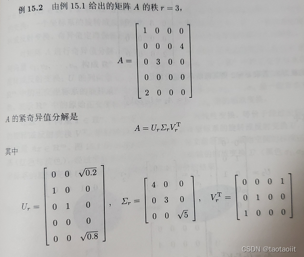
代码如下:
intmain(){
    vector<vector<double>> A ={{1,0,0,0},{0,0,0,4},{0,3,0,0},{0,0,0,0},{2,0,0,0}};
    SVD svd(A);// tight SVD
    svd.tight_svd();
    cout<<endl;
    cout<<"matrix A:"<<endl;display_matrix(A);
    cout<<endl;
    cout<<"matrix U:"<<endl;display_matrix(svd.U);
    cout<<endl;
    cout<<"matrix Sigma:"<<endl;display_matrix(svd.S);
    cout<<endl;
    cout<<"matrix V':"<<endl;display_matrix(transpose(svd.V));//display_matrix(matrix_multiply(matrix_multiply(svd.U,svd.S),transpose(svd.V)));//合成A}
测试结果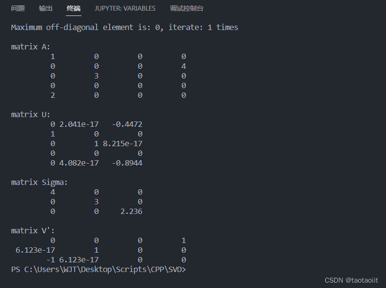
完整代码见我的GitHub仓库:https://github.com/wjtgoo/SVD-CPP(万水千山总是情,给个星星行不行/(ㄒoㄒ)/~~)
本文转载自: https://blog.csdn.net/weixin_45804601/article/details/125237191
版权归原作者 taotaoiit 所有, 如有侵权,请联系我们删除。
版权归原作者 taotaoiit 所有, 如有侵权,请联系我们删除。