
Pandas DataFrame 是一个包含二维数据及其对应索引的结构。DataFrame 广泛用于数据科学、机器学习、科学计算和许多其他数据密集型领域。
DataFrame 类似于SQL 表或在 Excel 中使用的电子表格。在许多情况下DataFrame 比表格或电子表格更快、更易于使用且功能更强大。

文章目录
Pandas DataFrame
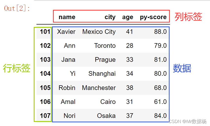
Pandas DataFrame 是包含以二维、行和列组织的数据、对应于行和列的索引的数据结构。
例如构建一个面试求职者的数据框。其中列数据包含姓名、城市、年龄和笔试分数。
-namecityagepy-score101XavierMexico City4188.0102AnnToronto2879.0103JanaPrague3381.0104YiShanghai3480.0105RobinManchester3868.0106AmalCairo3161.0107NoriOsaka3784.0
使用字典的方式创建DataFrame。
import pandas as pd

data ={'name':['Xavier','Ann','Jana','Yi','Robin','Amal','Nori'],'city':['Mexico City','Toronto','Prague','Shanghai','Manchester','Cairo','Osaka'],'age':[41,28,33,34,38,31,37],'py-score':[88.0,79.0,81.0,80.0,68.0,61.0,84.0]}

row_labels =[101,102,103,104,105,106,107]

df = pd.DataFrame(data=data, index=row_labels)
设定条件查询数据的前 N 行或者后 N 行内容。
df.head(2)
       name         city  age  py-score
101  Xavier  Mexico City   4188.0102     Ann      Toronto   2879.0
df.tail(2)
     name   city  age  py-score
106  Amal  Cairo   3161.0107  Nori  Osaka   3784.0
查看某列数据的话直接使用字典取值的方式获取即可。
cities = df['city']
cities

101    Mexico City
102        Toronto
103         Prague
104       Shanghai
105     Manchester
106          Cairo
107          Osaka
Name: city, dtype:object
也可以像获取类实例的属性一样访问该列数据。
df.city
101    Mexico City
102        Toronto
103         Prague
104       Shanghai
105     Manchester
106          Cairo
107          Osaka
Name: city, dtype:object
上面两种方法对比一下获取的数据是一样的。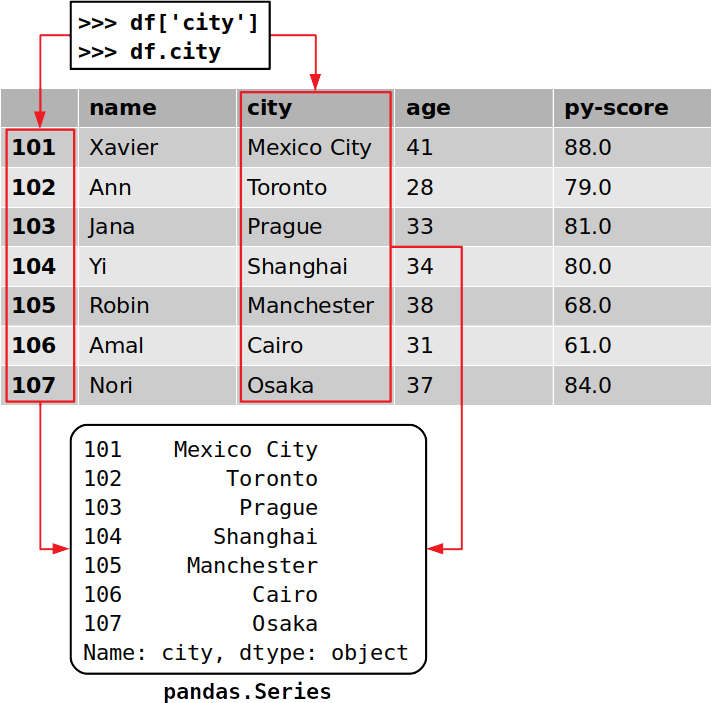
Pandas DataFrame 的每一列都是一个 pandas.Series 实例,保存一维数据及其索引的结构。可以像使用字典一样获取对象的单个项目,Series 方法是使用其索引作为键。
cities[102]'Toronto'
可以使用 .loc[] 访问器访问整行数据。
df.loc[103]
name          Jana
city        Prague
age             33
py-score        81
Name:103, dtype:objecttype(df.loc[103])
pandas.core.series.Series
label 对应的行103,其中包含对应行数据之外,还提取了相应列的索引,返回的行也是一个 pandas.Series 实例。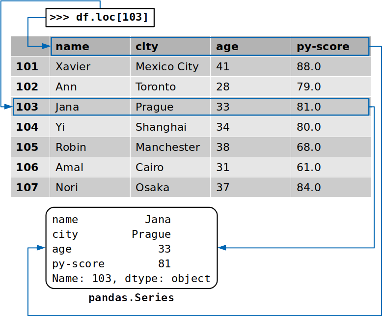
创建 DataFrame
分别使用不同的方式创建DataFrame,创建之前先要导入对应的三方库。
import numpy as np
import pandas as pd
使用 Dict 创建
data ={'x':[1,2,3],'y': np.array([2,4,8]),'z':100}
pd.DataFrame(data)

   x  y    z
012100124100238100
可以用 columns参数控制列的顺序,用index控制行索引的顺序。
pd.DataFrame(d, index=[100,200,300], columns=['z','y','x'])
       z  y  x
100100212001004230010083
使用 List 创建
字典键是列索引,字典值是 DataFrame 中的数据值。
l =[{'x':1,'y':2,'z':100},{'x':2,'y':4,'z':100},{'x':3,'y':8,'z':100}]

pd.DataFrame(l)
   x  y    z
012100124100238100
还可以使用嵌套列表或列表列表作为数据值,并且创建时需要指明行、列索引。元组和列表创建的方式相同。
l =[[1,2,100],[2,4,100],[3,8,100]]

pd.DataFrame(l, columns=['x','y','z'])
   x  y    z
012100124100238100
使用 NumPy 数组创建
arr = np.array([[1,2,100],[2,4,100],[3,8,100]])

df_ = pd.DataFrame(arr, columns=['x','y','z'])
df_
   x  y    z
012100124100238100
文件读取创建
可以在多种文件类型(包括 CSV、Excel、SQL、JSON 等)中保存和加载Pandas DataFrame 中的数据和索引。
先将生成的数据保存到不同的文件中。
import pandas as pd

data ={'name':['Xavier','Ann','Jana','Yi','Robin','Amal','Nori'],'city':['Mexico City','Toronto','Prague','Shanghai','Manchester','Cairo','Osaka'],'age':[41,28,33,34,38,31,37],'py-score':[88.0,79.0,81.0,80.0,68.0,61.0,84.0]}

row_labels =[101,102,103,104,105,106,107]

df = pd.DataFrame(data=data, index=row_labels)

df.to_csv('data.csv')
df.to_excel('data.xlsx')
检索索引和数据
创建 DataFrame 后可以进行一些检索、修改操作。
索引作为序列
df.index
Int64Index([1,2,3,4,5,6,7], dtype='int64')

df.columns
Index(['name','city','age','py-score'], dtype='object')

df.columns[1]'city'
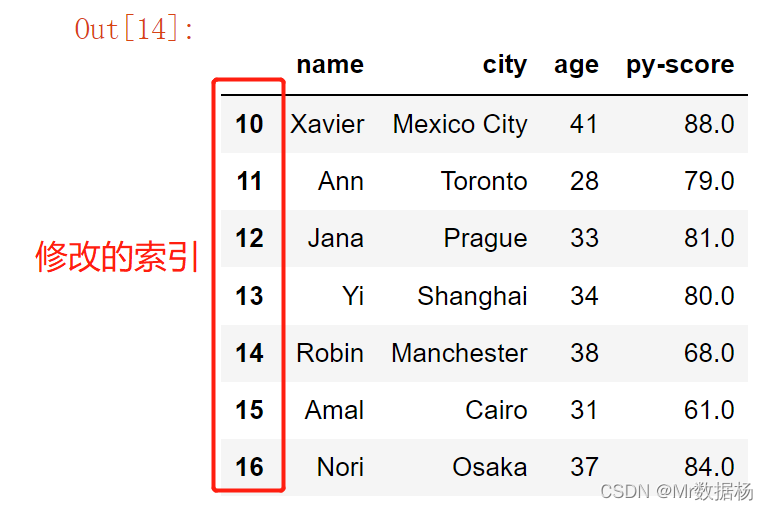
用序列修改索引。
df.index = np.arange(10,17)

df.index
Int64Index([10,11,12,13,14,15,16], dtype='int64')

df
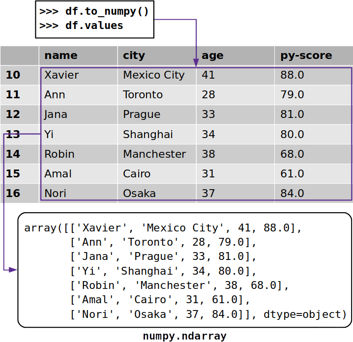
数据转为 NumPy 数组
转化之后取值方式同List操作。
df.to_numpy()
array([['Xavier','Mexico City',41,88.0],['Ann','Toronto',28,79.0],['Jana','Prague',33,81.0],['Yi','Shanghai',34,80.0],['Robin','Manchester',38,68.0],['Amal','Cairo',31,61.0],['Nori','Osaka',37,84.0]], dtype=object)
数据类型
数据值的类型,也称为数据类型或 dtypes,决定了 DataFrame 使用的内存量,以及计算速度和精度水平。
查看数据类型。
df.dtypes
name         object
city         object
age           int64
py-score    float64
dtype:object
使用.astype() 更改数据类型。
df_ = df.astype(dtype={'age': np.int32,'py-score': np.float32})
df_.dtypes
name         object
city         object
age           int32
py-score    float32
dtype:object
DataFrame 大小
.ndim、.size和.shape分别返回维度数、每个维度上的数据值数和数据值总数。
df_.ndim
2

df_.shape
(7,4)

df_.size
28
访问和修改数据
使用访问器获取数据
除了.loc[] 可以使用通过索引获取行或列的访问器之外,Pandas 还提供了访问器.iloc[],它通过整数索引检索行或列。
df.loc[10]
name             Xavier
city        Mexico City
age                  41
py-score             88
Name:10, dtype:object

df.iloc[0]
name             Xavier
city        Mexico City
age                  41
py-score             88
Name:10, dtype:object
.loc[] 和 .iloc[] 支持切片和 NumPy 的索引操作。
df.loc[:,'city']10    Mexico City
11        Toronto
12         Prague
13       Shanghai
14     Manchester
15          Cairo
16          Osaka
Name: city, dtype:object

df.iloc[:,1]10    Mexico City
11        Toronto
12         Prague
13       Shanghai
14     Manchester
15          Cairo
16          Osaka
Name: city, dtype:object
提供切片以及列表或数组而不是索引来获取多行或多列。
df.loc[11:15,['name','city']]
     name        city
11    Ann     Toronto
12   Jana      Prague
13     Yi    Shanghai
14  Robin  Manchester
15   Amal       Cairo

df.iloc[1:6,[0,1]]
     name        city
11    Ann     Toronto
12   Jana      Prague
13     Yi    Shanghai
14  Robin  Manchester
15   Amal       Cairo
.iloc[] 使用与切片元组、列表和 NumPy 数组相同的方式跳过行和列。
df.iloc[1:6:2,0]11     Ann
13      Yi
15    Amal
Name: name, dtype:object
使用 Python 内置的 **slice()**类,numpy.s_[] 或者 pd.IndexSlice[]。
df.iloc[slice(1,6,2),0]11     Ann
13      Yi
15    Amal
Name: name, dtype:object

df.iloc[np.s_[1:6:2],0]11     Ann
13      Yi
15    Amal
Name: name, dtype:object

df.iloc[pd.IndexSlice[1:6:2],0]11     Ann
13      Yi
15    Amal
Name: name, dtype:object
使用 .loc[] 和 .iloc[] 获取特定的数据值。但只需要一个值时建议使用专门的访问器 .at[] 和 .iat[]。
df.at[12,'name']'Jana'

df.iat[2,0]'Jana'
使用访问器设置数据
可以使用访问器通过传递 Python 序列、NumPy 数组或单个值来修改数据。
df.loc[:,'py-score']1088.01179.01281.01380.01468.01561.01684.0
Name: py-score, dtype: float64

df.loc[:13,'py-score']=[40,50,60,70]
df.loc[14:,'py-score']=0

df['py-score']1040.01150.01260.01370.0140.0150.0160.0
Name: py-score, dtype: float64
使用负索引 .iloc[] 来访问或修改数据。
df.iloc[:,-1]= np.array([88.0,79.0,81.0,80.0,68.0,61.0,84.0])>>> df['py-score']1088.01179.01281.01380.01468.01561.01684.0
Name: py-score, dtype: float64
插入和删除数据
Pandas 提供了几种方便的方法来插入和删除行或列。
插入和删除行
创建一个插入的新数据。
john = pd.Series(data=['John','Boston',34,79],index=df.columns, name=17)
john
name          John
city        Boston
age             34
py-score        79
Name:17, dtype:object
使用 df.append() 加入新的数据。
df = df.append(john)
df
      name         city  age  py-score
10  Xavier  Mexico City   4188.011     Ann      Toronto   2879.012    Jana       Prague   3381.013      Yi     Shanghai   3480.014   Robin   Manchester   3868.015    Amal        Cairo   3161.016    Nori        Osaka   3784.017    John       Boston   3479.0
使用 df.drop() 删除新的数据。
df = df.drop(labels=[17])
df
      name         city  age  py-score
10  Xavier  Mexico City   4188.011     Ann      Toronto   2879.012    Jana       Prague   3381.013      Yi     Shanghai   3480.014   Robin   Manchester   3868.015    Amal        Cairo   3161.016    Nori        Osaka   3784.0
插入和删除列
直接赋值定义列名和定义数据。
df['js-score']= np.array([71.0,95.0,88.0,79.0,91.0,91.0,80.0])
df
      name         city  age  py-score  js-score
10  Xavier  Mexico City   4188.071.011     Ann      Toronto   2879.095.012    Jana       Prague   3381.088.013      Yi     Shanghai   3480.079.014   Robin   Manchester   3868.091.015    Amal        Cairo   3161.091.016    Nori        Osaka   3784.080.0

df['total-score']=0.0
df
      name         city  age  py-score  js-score  total-score
10  Xavier  Mexico City   4188.071.00.011     Ann      Toronto   2879.095.00.012    Jana       Prague   3381.088.00.013      Yi     Shanghai   3480.079.00.014   Robin   Manchester   3868.091.00.015    Amal        Cairo   3161.091.00.016    Nori        Osaka   3784.080.00.0
.insert() 在列的指定位置插入列数据。
df.insert(loc=4, column='django-score',value=np.array([86.0,81.0,78.0,88.0,74.0,70.0,81.0]))
df
      name         city  age  py-score  django-score  js-score  total-score
10  Xavier  Mexico City   4188.086.071.00.011     Ann      Toronto   2879.081.095.00.012    Jana       Prague   3381.078.088.00.013      Yi     Shanghai   3480.088.079.00.014   Robin   Manchester   3868.074.091.00.015    Amal        Cairo   3161.070.091.00.016    Nori        Osaka   3784.081.080.00.0
del 删除一列或者多列。
del df['total-score']
df
      name         city  age  py-score  django-score  js-score
10  Xavier  Mexico City   4188.086.071.011     Ann      Toronto   2879.081.095.012    Jana       Prague   3381.078.088.013      Yi     Shanghai   3480.088.079.014   Robin   Manchester   3868.074.091.015    Amal        Cairo   3161.070.091.016    Nori        Osaka   3784.081.080.0
使用 df.drop() 删除列。
df = df.drop(labels='age', axis=1)
df
      name         city  py-score  django-score  js-score
10  Xavier  Mexico City      88.086.071.011     Ann      Toronto      79.081.095.012    Jana       Prague      81.078.088.013      Yi     Shanghai      80.088.079.014   Robin   Manchester      68.074.091.015    Amal        Cairo      61.070.091.016    Nori        Osaka      84.081.080.0
应用算术运算
应用基本的算术运算。
df['py-score']+ df['js-score']10159.011174.012169.013159.014159.015152.016164.0
dtype: float64

df['py-score']/100100.88110.79120.81130.80140.68150.61160.84
Name: py-score, dtype: float64
线性组合公式计算汇总数据。
df['total']=0.4* df['py-score']+0.3* df['django-score']+0.3* df['js-score']
df
      name         city  py-score  django-score  js-score  total
10  Xavier  Mexico City      88.086.071.082.311     Ann      Toronto      79.081.095.084.412    Jana       Prague      81.078.088.082.213      Yi     Shanghai      80.088.079.082.114   Robin   Manchester      68.074.091.076.715    Amal        Cairo      61.070.091.072.716    Nori        Osaka      84.081.080.081.9
应用 NumPy 和 SciPy 函数
大多数 NumPy 和 SciPy 都可以作为参数而不是 NumPy 数组应用于 Pandas Series 或 DataFrame 对象。 可以使用 NumPy 的 numpy.average() 计算考生的总考试成绩。
import numpy as np

score = df.iloc[:,2:5]
score
    py-score  django-score  js-score
1088.086.071.01179.081.095.01281.078.088.01380.088.079.01468.074.091.01561.070.091.01684.081.080.0

np.average(score, axis=1,weights=[0.4,0.3,0.3])
array([82.3,84.4,82.2,82.1,76.7,72.7,81.9])
del df['total']
df['total']= np.average(df.iloc[:,2:5], axis=1,weights=[0.4,0.3,0.3])
df
      name         city  py-score  django-score  js-score  total
10  Xavier  Mexico City      88.086.071.082.311     Ann      Toronto      79.081.095.084.412    Jana       Prague      81.078.088.082.213      Yi     Shanghai      80.088.079.082.114   Robin   Manchester      68.074.091.076.715    Amal        Cairo      61.070.091.072.716    Nori        Osaka      84.081.080.081.9
DataFrame 进行排序
.sort_values() 进行数据排序,需要指定排序的列。
df.sort_values(by='js-score', ascending=False)
      name         city  py-score  django-score  js-score  total
11     Ann      Toronto      79.081.095.084.414   Robin   Manchester      68.074.091.076.715    Amal        Cairo      61.070.091.072.712    Jana       Prague      81.078.088.082.216    Nori        Osaka      84.081.080.081.913      Yi     Shanghai      80.088.079.082.110  Xavier  Mexico City      88.086.071.082.3
也可以指定多个列和多个列的排序方式。
df.sort_values(by=['total','py-score'], ascending=[False,False])
      name         city  py-score  django-score  js-score  total
11     Ann      Toronto      79.081.095.084.410  Xavier  Mexico City      88.086.071.082.312    Jana       Prague      81.078.088.082.213      Yi     Shanghai      80.088.079.082.116    Nori        Osaka      84.081.080.081.914   Robin   Manchester      68.074.091.076.715    Amal        Cairo      61.070.091.072.7
DataFrame 过滤数据
Pandas 的过滤功能工作方式类似于在 NumPy 中使用布尔数组进行索引。
filter_ = df['django-score']>=80
filter_
10True11True12False13True14False15False16True
Name: django-score, dtype:bool
使用表达式 df[filter_] 返回一个 DataFrame 中 True 的行数据。
df[filter_]
      name         city  py-score  django-score  js-score  total
10  Xavier  Mexico City      88.086.071.082.311     Ann      Toronto      79.081.095.084.413      Yi     Shanghai      80.088.079.082.116    Nori        Osaka      84.081.080.081.9
可是使用逻辑运算进行多条件的筛选。
df[(df['py-score']>=80)&(df['js-score']>=80)]
    name    city  py-score  django-score  js-score  total
12  Jana  Prague      81.078.088.082.216  Nori   Osaka      84.081.080.081.9
使用.where() 可以替换不满足所提供条件的位置的值。
df['django-score'].where(cond=df['django-score']>=80, other=0.0)1086.01181.0120.01388.0140.0150.01681.0
Name: django-score, dtype: float64
DataFrame 数据统计
基本统计信息使用 **.describe()**。
df.describe()
        py-score  django-score   js-score      total
count   7.0000007.0000007.0000007.000000
mean   77.28571479.71428685.00000080.328571
std     9.4465926.3433508.5440044.101510min61.00000070.00000071.00000072.70000025%73.50000076.00000079.50000079.30000050%80.00000081.00000088.00000082.10000075%82.50000083.50000091.00000082.250000max88.00000088.00000095.00000084.400000
特定统计信息可以直接进行索引方法调用。
df.mean()
py-score        77.285714
django-score    79.714286
js-score        85.000000
total           80.328571
dtype: float64

df['py-score'].mean()77.28571428571429

df.std()
py-score        9.446592
django-score    6.343350
js-score        8.544004
total           4.101510
dtype: float64

df['py-score'].std()9.446591726019244
DataFrame 处理缺失数据
缺失数据在数据科学和机器学习中非常常见。Pandas 具有非常强大的处理缺失数据的功能。
Pandas 通常用 NaN(不是数字)值表示缺失数据。 在 Python 中可以使用 float(‘nan’)、math.nan 或 numpy.nan 获取 NaN。 从 Pandas 1.0 开始BooleanDtype、Int8Dtype、Int16Dtype、Int32Dtype 和 Int64Dtype 等新类型使用 pandas.NA 作为缺失值。
df_ = pd.DataFrame({'x':[1,2, np.nan,4]})
df_
     x
01.012.02  NaN
34.0
缺失数据进行计算
许多 Pandas 方法在执行计算时会忽略 nan 值,除非明确指示。
df_.mean()
x    2.333333
dtype: float64

df_.mean(skipna=False)
x   NaN
dtype: float64
填充缺失数据
.fillna() 进行缺失数据填充。
# 指定填充数据
df_.fillna(value=0)
     x
01.012.020.034.0# 向前填充
df_.fillna(method='ffill')
     x
01.012.022.034.0# 向后填充
df_.fillna(method='bfill')
     x
01.012.024.034.0
删除缺少数据的行和列
使用 .dropna() 直接进行处理。
df_.dropna()
     x
01.012.034.0
遍历 DataFrame
使用.items()and .iteritems() 遍历 Pandas DataFrame 的列。每次迭代都会产生一个以列名和列数据作为Series对象的元组。
for col_label, col in df.iteritems():print(col_label, col, sep='\n', end='\n\n')

name
10    Xavier
11       Ann
12      Jana
13        Yi
14     Robin
15      Amal
16      Nori
Name: name, dtype:object

city
10    Mexico City
11        Toronto
12         Prague
13       Shanghai
14     Manchester
15          Cairo
16          Osaka
Name: city, dtype:object

py-score
1088.01179.01281.01380.01468.01561.01684.0
Name: py-score, dtype: float64

django-score
1086.01181.01278.01388.01474.01570.01681.0
Name: django-score, dtype: float64

js-score
1071.01195.01288.01379.01491.01591.01680.0
Name: js-score, dtype: float64

total
1082.31184.41282.21382.11476.71572.71681.9
Name: total, dtype: float64
使用 .iterrows() 遍历 DataFrame 的行。
for row_label, row in df.iterrows():print(row_label, row, sep='\n', end='\n\n')10
name                 Xavier
city            Mexico City
py-score                 88
django-score             86
js-score                 71
total                  82.3
Name:10, dtype:object11
name                Ann
city            Toronto
py-score             79
django-score         81
js-score             95
total              84.4
Name:11, dtype:object12
name              Jana
city            Prague
py-score            81
django-score        78
js-score            88
total             82.2
Name:12, dtype:object13
name                  Yi
city            Shanghai
py-score              80
django-score          88
js-score              79
total               82.1
Name:13, dtype:object14
name                 Robin
city            Manchester
py-score                68
django-score            74
js-score                91
total                 76.7
Name:14, dtype:object15
name             Amal
city            Cairo
py-score           61
django-score       70
js-score           91
total            72.7
Name:15, dtype:object16
name             Nori
city            Osaka
py-score           84
django-score       81
js-score           80
total            81.9
Name:16, dtype:object
DataFrame 时间序列
使用时间序列创建index
创建一个 一天中的每小时温度数据 DataFrame。
temp_c =[8.0,7.1,6.8,6.4,6.0,5.4,4.8,5.0,9.1,12.8,15.3,19.1,21.2,22.1,22.4,23.1,21.0,17.9,15.5,14.4,11.9,11.0,10.2,9.1]
使用 date_range() 构建时间索引。
dt = pd.date_range(start='2022-04-16 00:00:00.0', periods=24,freq='H')
df
DatetimeIndex(['2022-04-16 00:00:00','2022-04-16 01:00:00','2022-04-16 02:00:00','2022-04-16 03:00:00','2022-04-16 04:00:00','2022-04-16 05:00:00','2022-04-16 06:00:00','2022-04-16 07:00:00','2022-04-16 08:00:00','2022-04-16 09:00:00','2022-04-16 10:00:00','2022-04-16 11:00:00','2022-04-16 12:00:00','2022-04-16 13:00:00','2022-04-16 14:00:00','2022-04-16 15:00:00','2022-04-16 16:00:00','2022-04-16 17:00:00','2022-04-16 18:00:00','2022-04-16 19:00:00','2022-04-16 20:00:00','2022-04-16 21:00:00','2022-04-16 22:00:00','2022-04-16 23:00:00'],
              dtype='datetime64[ns]', freq='H')
使用日期时间值作为行索引很方便。
                    temp_c
2022-04-1600:00:008.02022-04-1601:00:007.12022-04-1602:00:006.82022-04-1603:00:006.42022-04-1604:00:006.02022-04-1605:00:005.42022-04-1606:00:004.82022-04-1607:00:005.02022-04-1608:00:009.12022-04-1609:00:0012.82022-04-1610:00:0015.32022-04-1611:00:0019.12022-04-1612:00:0021.22022-04-1613:00:0022.12022-04-1614:00:0022.42022-04-1615:00:0023.12022-04-1616:00:0021.02022-04-1617:00:0017.92022-04-1618:00:0015.52022-04-1619:00:0014.42022-04-1620:00:0011.92022-04-1621:00:0011.02022-04-1622:00:0010.22022-04-1623:00:009.1
索引和切片
用切片来获取部分信息。
temp["2022-04-16 02:00:00":"2022-04-16 08:00:00"]
                    temp_c
2022-04-1602:00:006.82022-04-1603:00:006.42022-04-1604:00:006.02022-04-1605:00:005.42022-04-1606:00:004.82022-04-1607:00:005.02022-04-1608:00:009.1
重采样
使用 .resample() 进行重采样选取数据。
temp.resample(rule='6h').mean()
                    temp_c
2022-04-1600:00:006.6166672022-04-1606:00:0011.0166672022-04-1612:00:0021.2833332022-04-1618:00:0012.016667
窗口滚动
使用 .rolling() 进行固定长度滚动窗口分析,指定数量的相邻行计算统计数据。
temp.rolling(window=3).mean()
temp_c
2022-04-1600:00:00    NaN
2022-04-1601:00:00    NaN
2022-04-1602:00:007.3000002022-04-1603:00:006.7666672022-04-1604:00:006.4000002022-04-1605:00:005.9333332022-04-1606:00:005.4000002022-04-1607:00:005.0666672022-04-1608:00:006.3000002022-04-1609:00:008.9666672022-04-1610:00:0012.4000002022-04-1611:00:0015.7333332022-04-1612:00:0018.5333332022-04-1613:00:0020.8000002022-04-1614:00:0021.9000002022-04-1615:00:0022.5333332022-04-1616:00:0022.1666672022-04-1617:00:0020.6666672022-04-1618:00:0018.1333332022-04-1619:00:0015.9333332022-04-1620:00:0013.9333332022-04-1621:00:0012.4333332022-04-1622:00:0011.0333332022-04-1623:00:0010.100000
DataFrame 绘图
Pandas 允许基于 DataFrames 可视化数据或创建绘图。它在后台使用Matplotlib ,因此利用 Pandas 的绘图功能与使用 Matplotlib 非常相似。
import matplotlib.pyplot as plt
temp.plot()
plt.show()
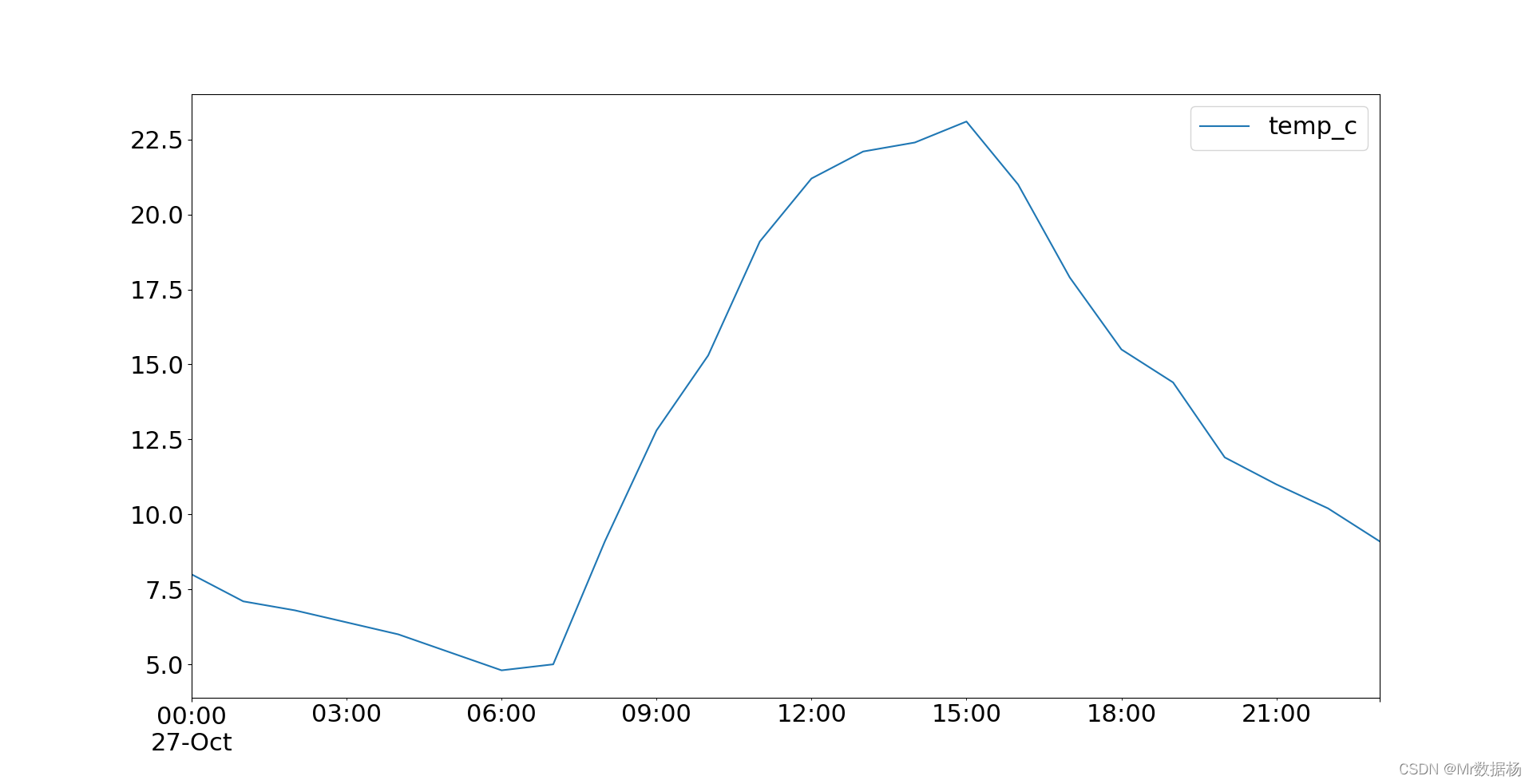
图像的保存。
temp.plot().get_figure().savefig('tmp.png')
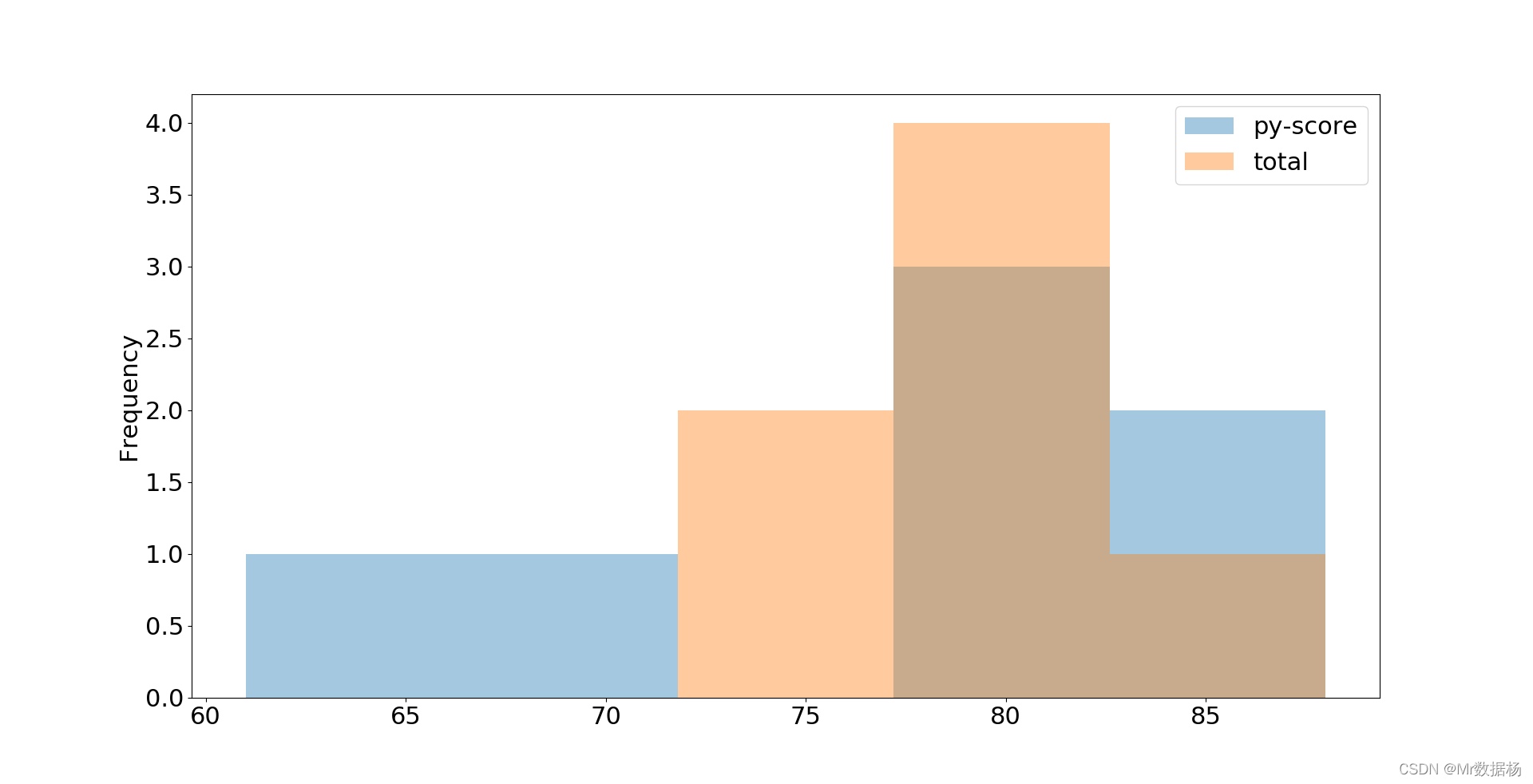
其他图表,比如直方图。
df.loc[:,['py-score','total']].plot.hist(bins=5, alpha=0.4)
plt.show()
版权归原作者 Mr数据杨 所有, 如有侵权,请联系我们删除。