
本文将介绍如何使用卷积操作实现因子分解机器。卷积网络因其局部性和权值共享的归纳偏差而在计算机视觉领域获得了广泛的成功和应用。卷积网络可以用来捕获形状的堆叠分类特征(B, num_cat, embedding_size)和形状的堆叠特征(B, num_features, embedding_size)之间的特征交互。
作为分解机的卷积网络
下图显示了卷积网络如何创建交互特征
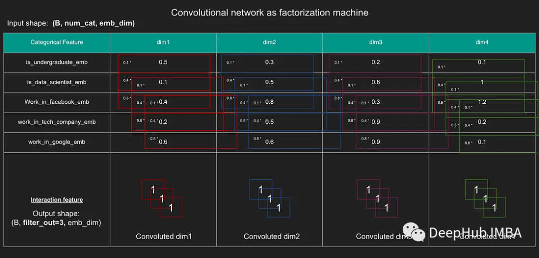
上图有5个已经进行嵌入的分类特征(batch_size, num_categorical=5, embedding_size)。假设我们有一个大小为(高度=3,宽度为1)的卷积过滤器。当我们在num_categorical维度(输入维度=1)上应用卷积(高度=3,宽度=1)的过滤器时,使用红框的示例(当我们在dim=1上卷积时),可以看到我们有效地计算了3个特征之间的卷积(因为过滤器的高度为3)。单个卷积的每个输出是3个分类特征之间的相互作用。当我们在num_categorical上滑动卷积时,可以有效地捕获任何滚动三元组特征之间的交互,其中3个不同特征窗口之间的每个交互都在卷积的输出中被捕获。
因为过滤器的宽度为1,所以正在计算三个特征在嵌入维度上独立的滚动窗口交互,如红色、蓝色、紫色和绿色框所示。卷积层的输出高度是产生的可能交互特征的总数,本例是3。卷积层输出的宽度将是原始嵌入大小,因为卷积滤波器的宽度为1。
由于嵌入大小是相同的,我们可以有效地将卷积网络的这种使用视为分解机,其中以滚动窗口的方式捕获特征之间的交互。
PyTorch实现
我们使用PyTorch进行实现,并且可视化视卷积网络中的填充、跨步和扩张
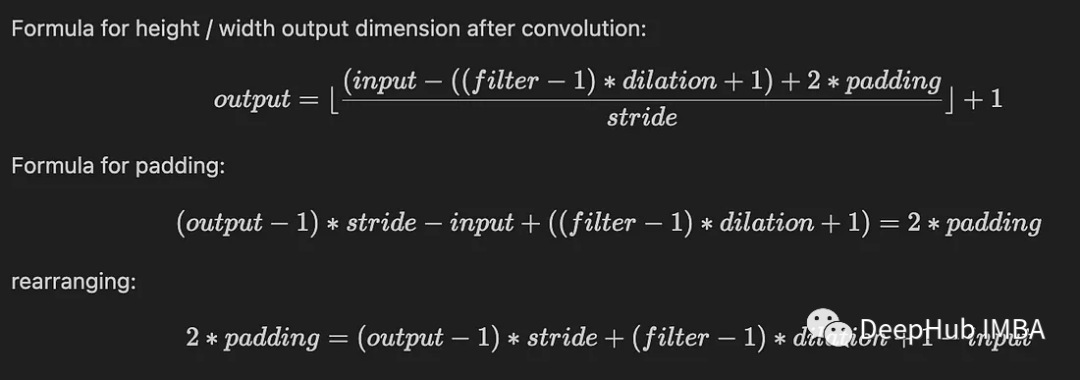
1、填充 Padding
进行填充后,我们的输入和输出的大小是相同的,下面代码在pytorch中使用padding='same'。
 class Conv2dSame(nn.Conv2d):
     def __init__(self, in_channels, out_channels, kernel_size, stride=1,
                  padding=0, dilation=1, groups=1, bias=True):
         # initialize with no padding first
         super(Conv2dSame, self).__init__(
             in_channels, out_channels, kernel_size, stride, 0, dilation,
             groups, bias)
         nn.init.xavier_uniform_(self.weight)
     def forward(self, x):
         # input height and width
         ih, iw = x.size()[-2:]
         # filter height and width
         kh, kw = self.weight.size()[-2:]
         # output height
         oh = math.ceil(ih / self.stride[0])
         # output width
         ow = math.ceil(iw / self.stride[1])
         # 2* padding for height
         pad_h = max((oh - 1) * self.stride[0] + (kh - 1) * self.dilation[0] + 1 - ih, 0)
         # 2 * padding for width
         pad_w = max((ow - 1) * self.stride[1] + (kw - 1) * self.dilation[1] + 1 - iw, 0)
         # divide the paddings equally on both sides and pad equally
         # note the ordering of the paddings are reversed for height and width. (it is width then height in the code)
         if pad_h > 0 or pad_w > 0:
             x = F.pad(x, [pad_w // 2, pad_w - pad_w // 2, pad_h // 2, pad_h - pad_h // 2])

         # manually create padding
         out = F.conv2d(x, self.weight, self.bias, self.stride,
                        self.padding, self.dilation, self.groups)
         return out

 # self implementation
 conv_same = Conv2dSame(in_channels=1, out_channels=5, kernel_size=3, stride=1, dilation=2, padding=0)
 conv_same_out= conv_same(x)

 ## pytorch
 conv_same_pt = nn.Conv2d(in_channels=1, out_channels=5, kernel_size=3, stride=1, dilation=2, padding='same')
 conv_same_pt.weight = conv_same.weight
 conv_same_pt.bias = conv_same.bias
 conv_same_pt_out= conv_same_pt(x)

 assert torch.equal(conv_same_out, conv_same_pt_out) == True
为什么需要填充
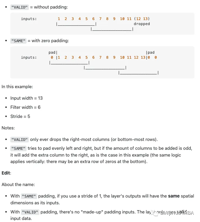
有两种最常见的填充类型:(1)“valid”填充(2)“same”填充,如上图所示。
使用“valid”填充对一个维度进行卷积时,输出维度将小于输入维度。(上面的“被丢弃”的例子)
使用“same”填充对一个维度进行卷积时,对输入数据进行填充,使输出维度与输入维度相同(参考上面的“pad”示例)。
2、步幅 Stride
步幅就是在输入上滑动过滤器的步长。
Stride指的是卷积核在输入张量上移动的步长:
步幅为1意味着过滤器每次移动一个元素,产生密集的计算。步幅大于1意味着过滤器在移动过程中跳过元素,产生输入的子采样。步幅直接影响输出特征图的空间维度。较大的步幅会导致输出大小的减小。
步幅为2,则输出大小将减小。我们可以用Pytorch验证这一点,如果我们将height和width的stride设置为2,则height和width从5减小到3。(注意,可以为高度和宽度指定不同的步长):
 # sample data
 batch_size=10
 channel_in = 1
 height = 5
 width = 5
 x = torch.randn(batch_size, channel_in, height, width)
 x.shape # torch.Size([10, 1, 5, 5])

 # padded convolution with padding specified in nn.Conv2d
 pad_conv = nn.Conv2d(in_channels=1, out_channels=5, kernel_size=3, stride=2, dilation=1, padding=1)
 pad_conv(x).shape # torch.Size([10, 5, 3, 3])
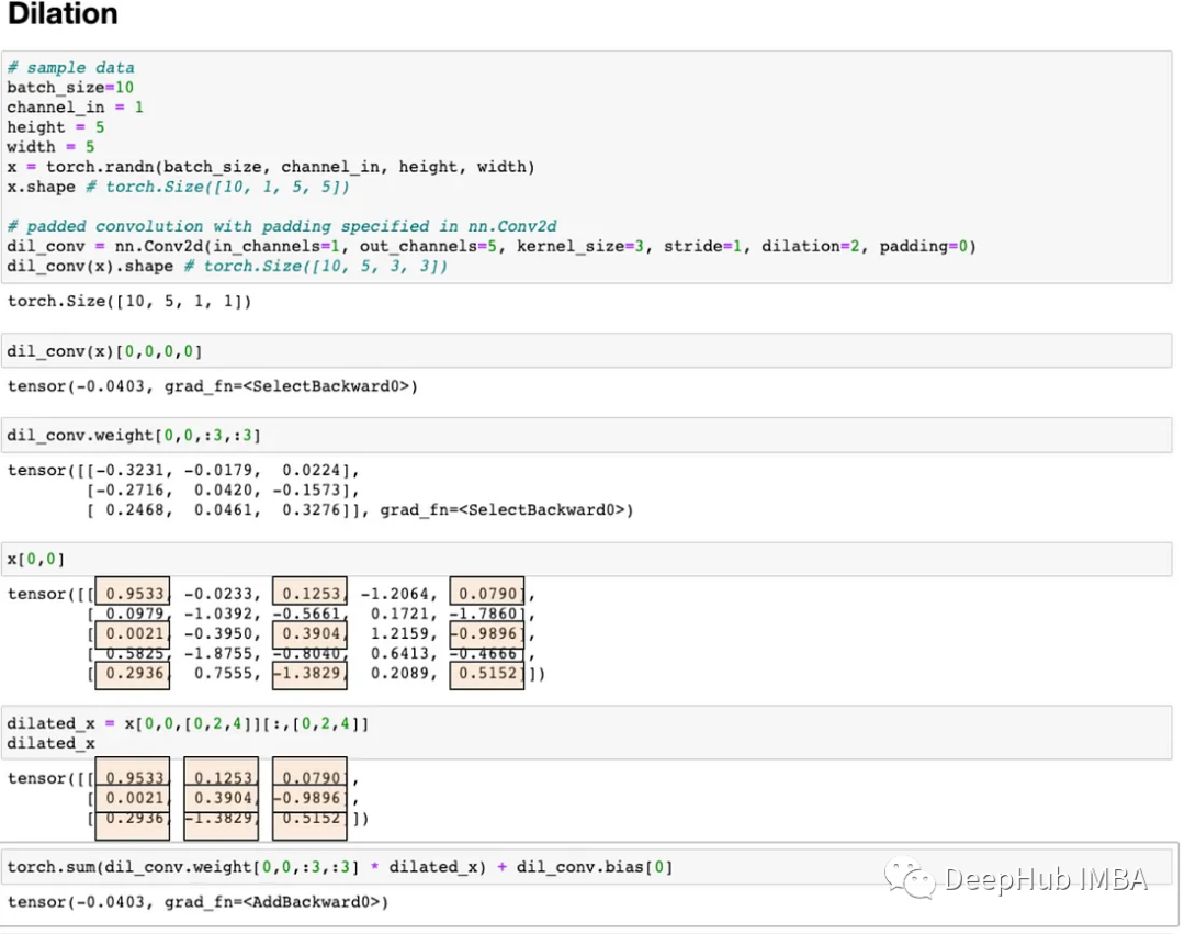
3、扩张 Dilation
扩张是滤波器中输入张量和权重之间的间隙大小
扩张是指卷积运算过程中核元素之间的间距。扩张为1意味着核元素之间没有间隙,产生标准卷积。大于1则引入了核元素之间的间隙,有效地扩展了卷积操作的接受域。
扩张通常用于增加卷积层的接受野,可以在不添加额外参数的情况下捕获更广泛的上下文信息。扩张不直接影响输出特征图的空间维度。它影响内核如何采样输入元素。
4、Flexible K-max pooling
在计算机视觉中,最大池化的思想已经非常流行,以减少卷积网络所需的计算,并已被证明是成功的识别图像中的重要特征。max_pooling在计算机视觉中表现得很好,但我们不能将其用于推荐系统,因为只检索(height, width)字段中的最大值是没有意义的,因为具有大值的交互特征将在池化层的输出中重复出现(由于卷积网络跨越输入的本质,其中每个输入可以在输出中出现多次)。
所以可以扩展池化操作(输出交互特征的大值比输出交互特征的小值更重要),并引入了灵活的p-max池化,只从每个卷积层输出中获得top-k个最大特征。因为k是由卷积层的深度决定的,它随着深度的增加而减小。这模仿了卷积层中的最大池化思想,其中最大池化产生的输出大小小于输入大小。
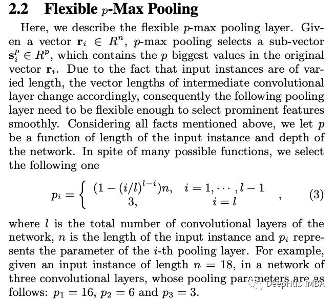
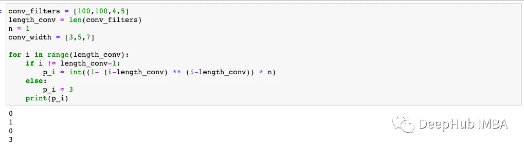
以上公式的代码如下:
 conv_filters = [100,100,4,5]
 length_conv = len(conv_filters)
 n = 10
 conv_width = [3,5,7]
 for i in range(length_conv):
     if i != length_conv-1:
         p_i = int((1- (i-length_conv) ** (i-length_conv)) * n)
     else:
         p_i = 3
     print(p_i)


 # 9
 # 10
 # 7
 # 3
这个公式并不完美。我们可以看到p_i的值通常趋向于减小。但是p_i可能会增加(例如,从9增加到10)。这就是为什么在代码中,我们必须确保p_i不会增加。如果我们设置n==1,也有可能p_i == 0。在使用时我们还需要在代码中处理这个问题
我们在Pytorch中实现k-max_pooling:根据number_of_feature的示例选择top-k个特征
 class KMaxPooling(nn.Module):
     """K Max pooling that selects the k biggest value along the specific axis.

       Input shape
         -  nD tensor with shape: ``(batch_size, ..., input_dim)``.

       Output shape
         - nD tensor with shape: ``(batch_size, ..., output_dim)``.

      """

     def __init__(self, k, axis, device='cpu'):
         super(KMaxPooling, self).__init__()
         self.k = k
         self.axis = axis
     def forward(self, inputs):
         out = torch.topk(inputs, k=self.k, dim=self.axis, sorted=True)[0]
         return out
5、因子分解机
有了以上的一些概念的介绍,我们就可以实现因子分解机了,我们将步骤分成3步:
(1)创建样本x,其中num_categories作为特征的数量
(2)根据层的深度计算p_i或k。
(3)使用k-max-Pooling得到当前conv层的最终输出
 # create sample
 batch_size=12
 num_categories = 10
 in_channel = 1 # must be 1 for it to work
 embedding_size = 11
 sample_x = torch.randn(batch_size, in_channel, num_categories, embedding_size)

 # initialize example
 conv_filters = [3,4,5]
 length_conv = len(conv_filters)
 n = num_categories
 conv_width = [3,5,7]
 field_shape = n
 module_list = []
 for i in range(1, length_conv+1):
     if i == 1:
         in_channels = 1
     else:
         in_channels = conv_filters[i-2]

     out_channels = conv_filters[i-1]
     width = conv_width[i-1]
     # max because it is possible that the formula is 0 if n == 1
     k = max(1, int((1- (i-length_conv) ** (i-length_conv)) * n)) if i < length_conv else 3
     #if i == 1,  shape = (B,out_channel, num_category, embedding_size)
     if i == 1:
         c = Conv2dSame(in_channels=in_channels, out_channels=out_channels, kernel_size=(width, 1), stride=1)
         first_out = c(sample_x)
         print(first_out.shape) # torch.Size([12, 3, 10, 11]) = (B,out_channel, num_category, embedding_size)
     module_list.append(Conv2dSame(in_channels=in_channels, out_channels=out_channels, kernel_size=(width, 1), stride=1))
     module_list.append(nn.ReLU())

     # get the topk values
     module_list.append(KMaxPooling(k=min(k, field_shape), axis=2)) # (B,out_channel, k, embedding_size)
     # we do not want the field_shape to increase
     field_shape = min(field_shape, k)

 conv_layer = nn.Sequential(*module_list)
 conv_layer(sample_x).shape
总结
我们首先介绍了卷积的一些基本知识,然后介绍了如何使用卷积实现因子分解机,因为使用来自卷积层的max_pooling来获得重要的交互特征是没有意义的,所以我们还介绍了一个新的池化层,然后将上面的内容整合完成了实现了因子分解机的操作。
本文的大部分内容来自于这篇论文:
http://wnzhang.net/share/rtb-papers/cnn-ctr.pdf
作者:Ngieng Kianyew