
TimesFM是一个为时间序列数据量身定制的大型预训练模型——一个无需大量再训练就能提供准确预测的模型。TimesFM有2亿参数,并在1000亿真实世界时间点上进行了训练。可以允许额外的协变量作为特征。
在本文中,我们将介绍模型架构、训练,并进行实际预测案例研究。将对TimesFM的预测能力进行分析,并将该模型与统计和机器学习模型进行对比。

TimesFM思路
用于时间序列预测的基础模型应能够适应不同的上下文和预测长度,同时具备足够的能力来编码来自广泛预训练数据集的所有模式。所以架构的住要办函如下内容:
1、分块 — 数据的分解
这个模型通过一个称为“分块”的过程,类似地处理时间序列数据。与一次性处理整个序列不同,它将数据分成更小、更易管理的片段,称为分块。这种方法不仅加快了模型的处理速度,还帮助它专注于数据中更小、更详细的趋势。
2、仅解码器架构
这个模型是在仅解码器模式下训练的。也就是说给定一系列输入分块,通过模型优化预测下一个分块作为所有过去分块的函数。类似于大型语言模型(LLMs),这可以在整个上下文窗口上并行完成,自动实现在观察到不同数量的输入分块后的未来预测。
3、生成较长的预测输出分块
在大型语言模型(LLMs)中,输出通常是以自回归方式逐个生成的。但是对于长期预测,一次性预测整个预测期可以比多步自回归解码获得更好的准确性。这种直接预测方法在预测期长度未知时(如零样本预测)尤为挑战,这是模型的主要关注点。
为了解决这个问题,作者建议通过使用比输入分块更长的输出分块来进行预测。例如,如果输入分块长度为32,输出分块长度为128,那么模型的训练方式如下:它使用前32个时间点来预测接下来的128个时间步,使用前64个时间点来预测第65到192个时间步,使用前96个时间点来预测第97到224个时间步,依此类推。
在推断时,如果模型接收到长度为256的新时间序列,并被要求预测接下来的256个时间步,它首先会预测第257到384个时间步。然后,它将使用初始的256长度输入以及生成的输出来预测第385到512个时间步。相比之下,输出分块长度等于输入分块长度的模型需要8个自回归步骤来完成相同的任务,而论文的方法只需要2个步骤。
但是这里有一个问题如果输出分块长度过长,处理短于输出分块长度的时间序列(如预训练数据中的月度或年度时间序列)会变得困难。
TimesFM模型架构
1、输入
- 时间序列经过预处理,被分割成连续的非重叠分块。
- 分块通过残差块处理,转换为大小为模型维度(model_dim)的向量。
- 二进制掩码也随输入一起提供给Transformer。二进制掩码用于表示相应的数据点是否应该被考虑(0)或忽略(1)。
- 残差块本质上是一个多层感知机块,具有一个带有跳跃连接的隐藏层。
2、Transformer架构
这个基础模型采用了堆叠Transformer的方法,每个Transformer层由两个主要组件组成:多头自注意力机制和前馈神经网络。
多头自注意力机制:每个Transformer层使用多头自注意力机制,允许模型同时关注输入序列的不同部分。这意味着对于给定的输出标记,模型可以同时考虑前面标记的多个方面,增强其捕捉数据中复杂模式和依赖关系的能力。
前馈网络:在自注意力机制之后,每个层对序列中的每个位置独立应用一个前馈网络。这进一步处理了注意力的信息,并使模型能够学习更高级别的表示。
因果注意力:在时间序列预测的背景下,作者实现了因果注意力。这确保每个输出标记只能关注其前面的标记。通过这样做,模型遵循数据的时间顺序,防止来自未来标记的信息(在预测时不应该可用)影响当前预测。
层堆叠:通过堆叠多个Transformer层,模型可以逐步构建输入数据的更抽象表示。每一层都会优化前几层学到的表示,使模型能够捕捉不同时间跨度上的复杂模式。
这包括两个关键超参数;
- 模型维度(Model Dimension):确定每个Transformer层中表示空间的大小。
- 注意力头的数量(Number of Attention Heads):指定模型可以同时关注输入的不同方面的数量。

如上所示的TimesFM体系结构采用特定长度的输入时间序列,并将其分解为多个输入片段。然后通过模型定义中定义的残差块将每个patch处理成一个向量,以匹配Transformer层的模型尺寸。然后将向量添加到位置编码中。具有位置编码的向量被发送到堆叠的Transformer层中。
SA是指自注意力,也就是是多头因果注意力,FFN是指全连接层。输出令牌通过一个残差块映射到一个大小为output_patch_len的输出,它构成了模型最后一个输入patch之后的时间窗口的预测。
3、输出层
输出层的任务是将输出标记映射到预测。模型采用了仅解码器模式进行训练,这意味着每个输出标记应该预测跟随最后输入分块的时间序列部分。与许多其他时间序列预测模型不同,输入分块长度不必等于输出分块长度。这意味着模型可以基于输入分块的信息预测时间序列的较大部分。
4、损失函数
研究使用的损失函数是均方误差(MSE)。由于这项工作围绕点预测展开,因此使用MSE来计算训练损失是合理的。
5、训练
模型使用标准的小批量梯度下降方法进行仅解码器的训练。该方法为每个时间序列和跨多个时间序列处理时间窗口。
训练使用的掩码策略是一个独特的特性。对于批处理中的每个时间序列,随机选择一个介于0和p−1之间的数字r,其中p是分块长度。创建一个掩码向量m1:r,其中m1设置为1,其余为零。这样可以屏蔽掉第一个输入分块的一部分。这种策略确保模型能够处理从1到最大上下文长度的输入上下文长度。以下面的相关示例可以很好地解释这一点:
假设最大上下文长度为512,分块长度p为32,r=4。在第一个分块后,输出预测被优化为使用32-4=28个时间点后进行预测。然后,下一个分块被优化为28+32个时间点后进行预测,依此类推。对所有这些r值重复此过程确保了模型可以处理所有长达512的上下文长度。
训练好的模型随后可以使用自回归解码生成任何时段的预测。
训练数据集
作者使用多样化的数据集对TimesFM模型进行预训练,以确保捕捉广泛的时间模式。他们从多个来源获取数据,包括:
- Google Trends:提供了超过22,000个查询在15年(2007年至2022年)的小时、日和周粒度的搜索兴趣数据,总共约50亿个时间点。
- Wiki Pageviews:包括来自2012年到2023年的维基百科页面的每小时查看次数。这些数据集被聚合到日、周和月的级别,贡献了约300亿个时间点。
除了真实世界的数据外,作者还生成了合成数据,使用ARMA模型、季节模式和趋势生成了300万条合成时间序列,每条时间序列有2048个时间点。
其他真实世界数据源包括M4数据集、每小时和15分钟的电力数据以及小时交通数据。M4数据集提供了约10万条时间序列,而交通和电力数据提供了大量时间序列,进一步增强了模型的鲁棒性。
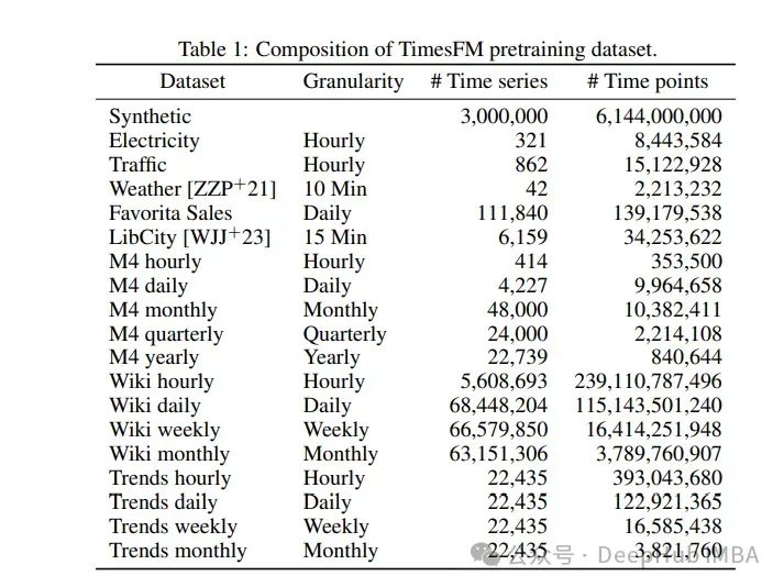
对于训练策略,作者创建了真实数据集和合成数据集的平衡组合,确保不同粒度(每小时、每天、每周、每月)的平等表示。训练批次从这些粒度中均匀取样,最小时间序列长度为256个时间点以保持一致性。时间序列按上下文均值和标准差进行缩放以标准化输入,每批包括15个主要时间序列。这种全面的方法确保了TimesFM模型为处理不同粒度的各种预测场景做好了充分准备。
代码示例对比
我们将介绍如何使用TimesFM模型进行预测。然后还会比较该模型与统计(AutoETS), ML(随机森林,XGBoost, LGBM)和其他的基础模型(TimeGPT)的性能。
本研究中使用的数据集取自Kaggle -每月黄金价格(1979-2021)- 18个不同国家的历史黄金价格
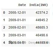
读取数据
 import pandas as pd
 df = pd.read_csv("GoldPrices.csv")
 df['Date'] = pd.to_datetime(df['Date'])
 df = df.set_index('Date').resample('MS').mean()
 df = df.reset_index() # Reset index to have 'Date' as a column again
 print(df.head())
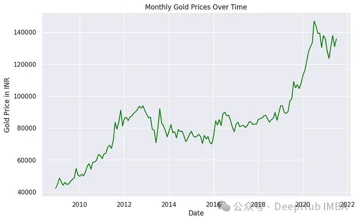
可视化
 #Let's Visualise the Dataset
 import matplotlib.pyplot as plt
 import seaborn as sns
 sns.set(style="darkgrid")
 plt.figure(figsize=(10, 6))
 sns.lineplot(x="Date", y='India(INR)', data=df, color='green')
 plt.title('Monthly Gold Prices Over Time')
 plt.xlabel('Date')
 plt.ylabel('Gold Price in INR')
 plt.show()
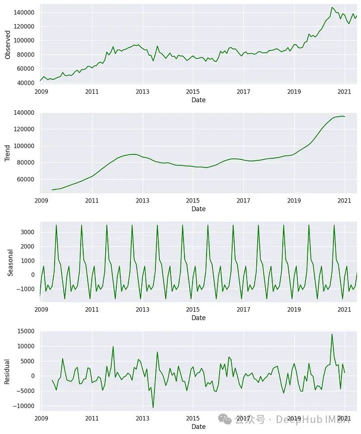
对数据进行季节性分解,检查这里的趋势和季节性模式。
 df.set_index("Date", inplace=True)
 from statsmodels.tsa.seasonal import seasonal_decompose

 result = seasonal_decompose(df['India(INR)'])

 fig, (ax1, ax2, ax3, ax4) = plt.subplots(4, 1, figsize=(10, 12))

 result.observed.plot(ax=ax1, color='green')
 ax1.set_ylabel('Observed')

 result.trend.plot(ax=ax2, color='green')
 ax2.set_ylabel('Trend')

 result.seasonal.plot(ax=ax3, color='green')
 ax3.set_ylabel('Seasonal')

 result.resid.plot(ax=ax4, color='green')
 ax4.set_ylabel('Residual')

 plt.tight_layout()
 plt.show()

 df.reset_index(inplace=True)
TimesFM期望数据在单变量时间序列数据中有三个不同的列。这些都是:
unique_id: unique_id列用于标识数据集中的不同时间序列。—可以是字符串、整数或分类类型。
它表示数据中每个时间序列的标识符。这在处理同一数据集中的多个时间序列时特别有用。
ds(日期戳):ds列表示时间序列数据的时间部分。-它应该是pandas可以解释为日期或时间戳的格式。
理想情况下,日期格式应为YYYY-MM-DD,时间戳格式应为YYYY-MM-DD HH:MM:SS。这对于MLForecast理解数据的时间方面至关重要。
y(目标变量):y想要预测的实际值。-应该是数字。这是想要预测的测量或数量。
df = pd.DataFrame({'unique_id':[1]*len(df),'ds': df["Date"], "y":df['India(INR)']})
然后进行训练-测试分割,我们将使用128个数据点用于训练,24个用于测试。
 train_df = df[df['ds'] <= '31-07-2019']
 test_df = df[df['ds'] > '31-07-2019']
1、统计预测
 #install statsforecast
 !pip install statsforecast

 import pandas as pd
 from statsforecast import StatsForecast
 from statsforecast.models import AutoARIMA, AutoETS

 # Define the AutoARIMA model
 autoarima = AutoARIMA(season_length=12)  # Annual seasonality for monthly data

 # Define the AutoETS model
 autoets = AutoETS(season_length=12)  # Annual seasonality for monthly data

 # Create StatsForecast object with AutoARIMA
 statforecast = StatsForecast(df=train_df,
                          models=[autoarima, autoets],
                          freq='MS',
                          n_jobs=-1)

 # Fit the model
 statforecast.fit()

 # Generate forecasts
 sf_forecast = statforecast.forecast(h=24)  # Forecasting for 24 periods
这些结果存储在sf_forecast中,我们后面展示
2、机器学习方法预测
 #install mlforecast
 !pip install mlforecast
 from mlforecast import MLForecast
 from mlforecast.target_transforms import AutoDifferences
 from numba import njit
 import lightgbm as lgb
 import xgboost as xgb
 from sklearn.ensemble import RandomForestRegressor
 from statsmodels.tsa.seasonal import seasonal_decompose
 from mlforecast import MLForecast
 from mlforecast.lag_transforms import (
     RollingMean, RollingStd, RollingMin, RollingMax, RollingQuantile,
     SeasonalRollingMean, SeasonalRollingStd, SeasonalRollingMin,
     SeasonalRollingMax, SeasonalRollingQuantile,
     ExpandingMean
 )

 models = [lgb.LGBMRegressor(verbosity=-1),  # LightGBM regressor with verbosity turned off
     xgb.XGBRegressor(),  # XGBoost regressor with default parameters
     RandomForestRegressor(random_state=0),  # Random Forest regressor with fixed random state for reproducibility
 ]
 fcst = MLForecast(
     models=models,  # List of models to be used for forecasting
     freq='MS',  # Monthly frequency, starting at the beginning of each month
     lags=[1,3,5,7,12],  # Lag features: values from 1, 3, 5, 7, and 12 time steps ago
     lag_transforms={
         1: [  # Transformations applied to lag 1
             RollingMean(window_size=3),  # Rolling mean with a window of 3 time steps
             RollingStd(window_size=3),  # Rolling standard deviation with a window of 3 time steps
             RollingMin(window_size=3),  # Rolling minimum with a window of 3 time steps
             RollingMax(window_size=3),  # Rolling maximum with a window of 3 time steps
             RollingQuantile(p=0.5, window_size=3),  # Rolling median (50th percentile) with a window of 3 time steps
             ExpandingMean()  # Expanding mean (mean of all previous values)
         ],
         6:[  # Transformations applied to lag 6
             RollingMean(window_size=6),  # Rolling mean with a window of 6 time steps
             RollingStd(window_size=6),  # Rolling standard deviation with a window of 6 time steps
             RollingMin(window_size=6),  # Rolling minimum with a window of 6 time steps
             RollingMax(window_size=6),  # Rolling maximum with a window of 6 time steps
             RollingQuantile(p=0.5, window_size=6),  # Rolling median (50th percentile) with a window of 6 time steps
         ],
         12: [  # Transformations applied to lag 12 (likely for yearly seasonality)
             SeasonalRollingMean(season_length=12, window_size=3),  # Seasonal rolling mean with 12-month seasonality and 3-month window
             SeasonalRollingStd(season_length=12, window_size=3),  # Seasonal rolling standard deviation with 12-month seasonality and 3-month window
             SeasonalRollingMin(season_length=12, window_size=3),  # Seasonal rolling minimum with 12-month seasonality and 3-month window
             SeasonalRollingMax(season_length=12, window_size=3),  # Seasonal rolling maximum with 12-month seasonality and 3-month window
             SeasonalRollingQuantile(p=0.5, season_length=12, window_size=3)  # Seasonal rolling median with 12-month seasonality and 3-month window
         ]
     },
     date_features=['year', 'month', 'quarter'],  # Extract year, month, and quarter from the date as features
     target_transforms=[AutoDifferences(max_diffs=3)])


 fcst.fit(train_df)
 ml_forecast = fcst.predict(len(test_df))
结果保存到ml_forecast
3、TimeGPT
 !pip install nixtla
 from nixtla import NixtlaClient
 # Get your API Key at dashboard.nixtla.io
 #Instantiate the NixtlaClient
 nixtla_client = NixtlaClient(api_key = 'Your_API_Key')
 #Get the forecast
 timegpt_forecast = nixtla_client.forecast(df = train_df, h=24, freq="M")
虽然TimeGPT已经被认为是一个笑话,但是我们还是要做下,如果TimesFM不如TimeGPT那说明他没有存在的意义。结果保存到timegpt_forecast
4、TimesFM
最后就是TimesFM模型,这是我们在这项研究中的主要兴趣点。
 !pip install timesfm #You might need to restart the kernal to have this installed in your w

 # Initialize the TimesFM model with specified parameters
 tfm = timesfm.TimesFm(
     context_len=128,       # Length of the context window for the model
     horizon_len=24,        # Forecasting horizon length
     input_patch_len=32,    # Length of input patches
     output_patch_len=128,  # Length of output patches
     num_layers=20,
     model_dims=1280,
 )

 # Load the pretrained model checkpoint
 tfm.load_from_checkpoint(repo_id="google/timesfm-1.0-200m")

 # Generate forecasts using the TimesFM model on the given DataFrame
 timesfm_forecast = tfm.forecast_on_df(
     inputs=train_df,       # Input DataFrame containing the time-series data for training
     freq="MS",             # Frequency of the time-series data (e.g., monthly start)
     value_name="y",        # Name of the column containing the values to be forecasted
     num_jobs=-1,           # Number of parallel jobs to use for forecasting (-1 uses all available cores)
 )
 timesfm_forecast = timesfm_forecast[["ds","timesfm"]]
这里面有一些超参数,应该还有优化的空间,不过我们先以这个进行测试。
最后我们还要把所有的日期转换成相同的格式,以解决格式不一致的问题
# Assuming the DataFrames have a common column 'ds' for the dates
# Convert 'ds' to datetime in all DataFrames if necessary
sf_forecast['ds'] = pd.to_datetime(sf_forecast['ds'])
ml_forecast['ds'] = pd.to_datetime(ml_forecast['ds'])
timegpt_forecast['ds'] = pd.to_datetime(timegpt_forecast['ds'])
timesfm_forecast['ds'] = pd.to_datetime(timesfm_forecast['ds'])
# Now perform the merges
merged_fcst = pd.merge(sf_forecast, ml_forecast, on='ds')
merged_fcst = pd.merge(merged_fcst, timegpt_forecast, on='ds')
merged_fcst = pd.merge(merged_fcst, timesfm_forecast, on='ds')
#Adding the actuals to the dataframe from test_df
merged_fcst = pd.merge(merged_fcst, test_df, on='ds')
#Keep only relevant columns
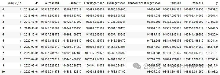
merged_fcst = merged_fcst[["unique_id", "ds", "AutoARIMA", "AutoETS", "LGBMRegressor", "XGBRegressor", "RandomForestRegressor", "TimeGPT", "timesfm"]]
所有的预测的结果如下:
最后就是评估我们的结果
 import numpy as np
 def calculate_error_metrics(actual_values, predicted_values):
     actual_values = np.array(actual_values)
     predicted_values = np.array(predicted_values)

     metrics_dict = {
         'MAE': np.mean(np.abs(actual_values - predicted_values)),
         'RMSE': np.sqrt(np.mean((actual_values - predicted_values)**2)),
         'MAPE': np.mean(np.abs((actual_values - predicted_values) / actual_values)) * 100
     }

     result_df = pd.DataFrame(list(metrics_dict.items()), columns=['Metric', 'Value'])
     return result_df

 # Extract 'Weekly_Sales' as actuals
 actuals = merged_fcst['y']

 error_metrics_dict = {}


 for col in merged_fcst.columns[2:-1]:  # Exclude 'Weekly_Sales'
     predicted_values = merged_fcst[col]
     error_metrics_dict[col] = calculate_error_metrics(actuals, predicted_values)['Value'].values  # Extracting 'Value' column


 error_metrics_df = pd.DataFrame(error_metrics_dict)
 error_metrics_df.insert(0, 'Metric', calculate_error_metrics(actuals, actuals)['Metric'].values)  # Adding 'Metric' column


 print(error_metrics_df)
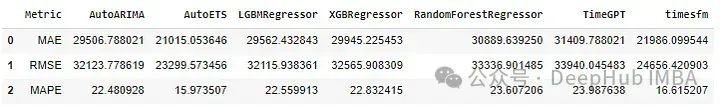
可以看出,在MAE、RMSE和MAPE的基础上进行比较,TimesFM是AutoETS之后最好的模型。
总结
TimesFM提供了一种可靠的时间序列基础模型方法,可以被考虑为我们工具箱中的一部分(无脑预测一波看看效果,作为基类模型对比)。TimesFM采用了仅解码器的Transformer架构,这与许多现有时间序列模型中使用的典型编码器-解码器框架形成对比。这种设计选择简化了模型,同时在预测任务中保持了高性能。正如研究所示,与另一个成功的时间序列基础模型——TimeGPT相比,TimesFM在这个实验案例中表现更好。
kaggle数据集:
https://www.kaggle.com/datasets/odins0n/monthly-gold-prices
本文处理后的数据集:
https://docs.google.com/spreadsheets/d/1BIbC_-rHtadBL6xzunKYOtKC0pNadqcH1eK4sFXRFBY/edit?usp=sharing
作者:Satyajit Chaudhuri