
本文的目的是提供代码示例,并解释使用python和TensorFlow建模时间序列数据的思路。
本文展示了如何进行多步预测并在模型中使用多个特征。
本文的简单版本是,使用过去48小时的数据和对未来1小时的预测(一步),我获得了温度误差的平均绝对误差0.48(中值0.34)度。
利用过去168小时的数据并提前24小时进行预测,平均绝对误差为摄氏温度1.69度(中值1.27)。
所使用的特征是过去每小时的温度数据、每日及每年的循环信号、气压及风速。
这里和整篇文章的主数据对象被称为d。它是通过读取原始数据创建的:
d = pd.read_csv(‘data/weather.csv’)
# Converting the dt column to datetime object
d[‘dt’] = [datetime.datetime.utcfromtimestamp(x) for x in d[‘dt’]]

# Sorting by the date
d.sort_values(‘dt’, inplace=True)
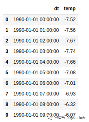

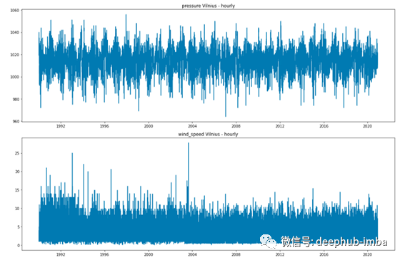
数据集中共有271008个数据点。

数据似乎是具有明确的周期模式。

上面的图表显示,气温有一个清晰的昼夜循环——中间温度在中午左右最高,在午夜左右最低。
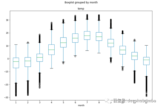
这种循环模式在按月份分组的温度上更为明显——最热的月份是6月到8月,最冷的月份是12月到2月。
数据现在的问题是,我们只有date列。如果将其转换为数值(例如,提取时间戳(以秒为单位))并将其作为建模时的特性添加,那么循环特性将丢失。因此,我们需要做的第一件事就是设计一些能够抓住周期性趋势的特性。
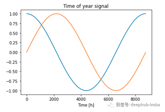
我们想让机器知道,23点和0点比小时0点和4点更接近。我们知道周期是24小时。我们可以用cos(x)和sin(x)函数。函数中的x是一天中的一个小时。
# Extracting the hour of day
d["hour"] = [x.hour for x in d["dt"]]

# Creating the cyclical daily feature
d["day_cos"] = [np.cos(x * (2 * np.pi / 24)) for x in d["hour"]]
d["day_sin"] = [np.sin(x * (2 * np.pi / 24)) for x in d["hour"]]
得到的dataframe如下:
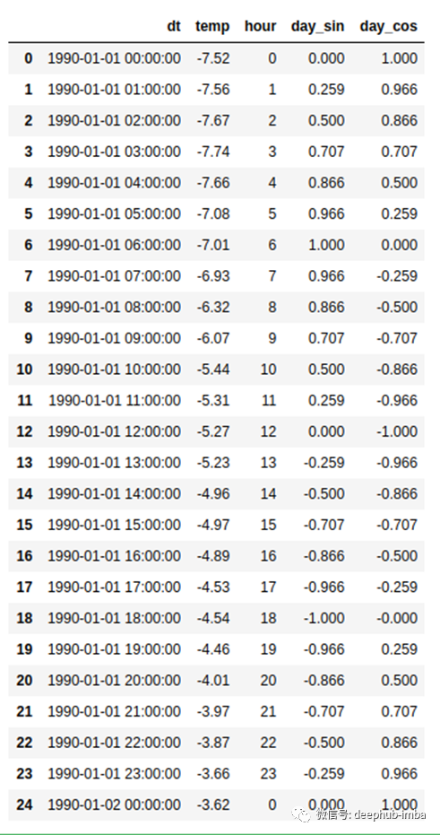
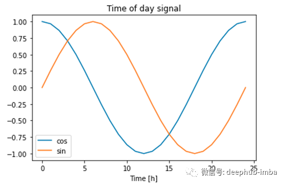
新创建的特征捕捉了周期性模式。可能会出现一个问题,为什么我们同时使用sin和cos函数?
在上图中绘制一条水平线并仅分析其中一条曲线,我们将得到例如cos(7.5h)= cos(17.5h)等。在学习和预测时,这可能会导致一些错误,因此为了使每个点都唯一,我们添加了另一个循环函数。同时使用这两个功能,可以将所有时间区分开。
为了在一年中的某个时间创建相同的循环逻辑,我们将使用时间戳功能。python中的时间戳是一个值,用于计算自1970.01.01 0H:0m:0s以来经过了多少秒。python中的每个date对象都具有timestamp()函数。
# Extracting the timestamp from the datetime object
d["timestamp"] = [x.timestamp() for x in d["dt"]]

# Seconds in day
s = 24 * 60 * 60

# Seconds in year
year = (365.25) * sd["month_cos"] = [np.cos((x) * (2 * np.pi / year)) for x in d["timestamp"]]
d["month_sin"] = [np.sin((x) * (2 * np.pi / year)) for x in d["timestamp"]]
在本节中,我们从datetime列中创建了4个其他功能:day_sin,day_cos,month_sin和month_cos。
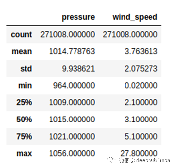
在天气数据集中,还有两列:wind_speed和pressure。风速以米/秒(m / s)为单位,压力以百帕斯卡(hPa)为单位。
要查看温度与两个特征之间的任何关系,我们可以绘制二维直方图:

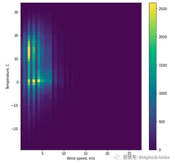
颜色越强烈,两个分布的某些bin值之间的关系就越大。例如,当压力在1010和1020 hPa左右时,温度往往会更高。
我们还将在建模中使用这两个功能。
我们使用所有要素工程获得的数据是:

我们要近似的函数f为:

目标是使用过去的值来预测未来。数据是时间序列或序列。对于序列建模,我们将选择具有LSTM层的递归神经网络的Tensorflow实现。
LSTM网络的输入是3D张量:
(样本,时间步长,功能)
样本—用于训练的序列总数。
timesteps-样本的长度。
功能-使用的功能数量。
建模之前的第一件事是将2D格式的数据转换为3D数组。以下功能可以做到这一点:
例如,如果我们假设整个数据是数据的前10行,那么我们将过去3个小时用作特征,并希望预测出1步:
def create_X_Y(ts: np.array, lag=1, n_ahead=1, target_index=0) -> tuple:
    """
    A method to create X and Y matrix from a time series array for the training of
    deep learning models
    """
    # Extracting the number of features that are passed from the array
    n_features = ts.shape[1]

    # Creating placeholder lists
    X, Y = [], []

    if len(ts) - lag <= 0:
        X.append(ts)
    else:
        for i in range(len(ts) - lag - n_ahead):
            Y.append(ts[(i + lag):(i + lag + n_ahead), target_index])
            X.append(ts[i:(i + lag)])

    X, Y = np.array(X), np.array(Y)

    # Reshaping the X array to an RNN input shape
    X = np.reshape(X, (X.shape[0], lag, n_features))

    return X, Y
例如,如果我们假设整个数据是数据的前10行,那么我们将过去3个小时用作特征,并希望预测出1步:
ts = d[
‘temp’,
‘day_cos’,
‘day_sin’,
‘month_sin’,
‘month_cos’,
‘pressure’,
‘wind_speed’].head(10).valuesX, Y = create_X_Y(ts, lag=3, n_ahead=1)

如我们所见,X矩阵的形状是6个样本,3个时间步长和7个特征。换句话说,我们有6个观测值,每个观测值都有3行数据和7列。之所以有6个观测值,是因为前3个滞后被丢弃并且仅用作X数据,并且我们预测提前1步,因此最后一个观测值也会丢失。
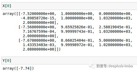
上图中显示了X和Y的第一个值对。
最终模型的超参数列表:
# Number of lags (hours back) to use for models
lag = 48

# Steps ahead to forecast
n_ahead = 1

# Share of obs in testing
test_share = 0.1

# Epochs for training
epochs = 20

# Batch size
batch_size = 512

# Learning rate
lr = 0.001

# Number of neurons in LSTM layer
n_layer = 10

# The features used in the modeling
features_final = [‘temp’, ‘day_cos’, ‘day_sin’, ‘month_sin’, ‘month_cos’, ‘pressure’, ‘wind_speed’]
模型代码
class NNMultistepModel():

    def __init__(
        self,
        X,
        Y,
        n_outputs,
        n_lag,
        n_ft,
        n_layer,
        batch,
        epochs,
        lr,
        Xval=None,
        Yval=None,
        mask_value=-999.0,
        min_delta=0.001,
        patience=5
    ):
        lstm_input = Input(shape=(n_lag, n_ft))

        # Series signal
        lstm_layer = LSTM(n_layer, activation='relu')(lstm_input)

        x = Dense(n_outputs)(lstm_layer)

        self.model = Model(inputs=lstm_input, outputs=x)
        self.batch = batch
        self.epochs = epochs
        self.n_layer=n_layer
        self.lr = lr
        self.Xval = Xval
        self.Yval = Yval
        self.X = X
        self.Y = Y
        self.mask_value = mask_value
        self.min_delta = min_delta
        self.patience = patience

    def trainCallback(self):
        return EarlyStopping(monitor='loss', patience=self.patience, min_delta=self.min_delta)

    def train(self):
        # Getting the untrained model
        empty_model = self.model

        # Initiating the optimizer
        optimizer = keras.optimizers.Adam(learning_rate=self.lr)

        # Compiling the model
        empty_model.compile(loss=losses.MeanAbsoluteError(), optimizer=optimizer)

        if (self.Xval is not None) & (self.Yval is not None):
            history = empty_model.fit(
                self.X,
                self.Y,
                epochs=self.epochs,
                batch_size=self.batch,
                validation_data=(self.Xval, self.Yval),
                shuffle=False,
                callbacks=[self.trainCallback()]
            )
        else:
            history = empty_model.fit(
                self.X,
                self.Y,
                epochs=self.epochs,
                batch_size=self.batch,
                shuffle=False,
                callbacks=[self.trainCallback()]
            )

        # Saving to original model attribute in the class
        self.model = empty_model

        # Returning the training history
        return history

    def predict(self, X):
        return self.model.predict(X)
创建用于建模之前的最后一步是缩放数据。
# Subseting only the needed columns
ts = d[features_final]nrows = ts.shape[0]

# Spliting into train and test sets
train = ts[0:int(nrows * (1 — test_share))]
test = ts[int(nrows * (1 — test_share)):]

# Scaling the data
train_mean = train.mean()
train_std = train.std()train = (train — train_mean) / train_std
test = (test — train_mean) / train_std

# Creating the final scaled frame
ts_s = pd.concat([train, test])

# Creating the X and Y for training
X, Y = create_X_Y(ts_s.values, lag=lag, n_ahead=n_ahead)n_ft = X.shape[2]
现在我们将数据分为训练和验证
# Spliting into train and test sets
Xtrain, Ytrain = X[0:int(X.shape[0] * (1 — test_share))], Y[0:int(X.shape[0] * (1 — test_share))]

Xval, Yval = X[int(X.shape[0] * (1 — test_share)):], Y[int(X.shape[0] * (1 — test_share)):]
数据的最终形状:
Shape of training data: (243863, 48, 7)
Shape of the target data: (243863, 1)
Shape of validation data: (27096, 48, 7)
Shape of the validation target data: (27096, 1)
剩下的就是使用模型类创建对象,训练模型并检查验证集中的结果。
# Initiating the model object
model = NNMultistepModel(
 X=Xtrain,
 Y=Ytrain,
 n_outputs=n_ahead,
 n_lag=lag,
 n_ft=n_ft,
 n_layer=n_layer,
 batch=batch_size,
 epochs=epochs,
 lr=lr,
 Xval=Xval,
 Yval=Yval,
)

# Training of the model
history = model.train()
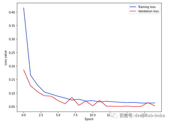
使用训练好的模型,我们可以预测值并将其与原始值进行比较。
# Comparing the forecasts with the actual values
yhat = [x[0] for x in model.predict(Xval)]
y = [y[0] for y in Yval]

# Creating the frame to store both predictions
days = d[‘dt’].values[-len(y):]frame = pd.concat([
 pd.DataFrame({‘day’: days, ‘temp’: y, ‘type’: ‘original’}),
 pd.DataFrame({‘day’: days, ‘temp’: yhat, ‘type’: ‘forecast’})
])

# Creating the unscaled values column
frame[‘temp_absolute’] = [(x * train_std[‘temp’]) + train_mean[‘temp’] for x in frame[‘temp’]]

# Pivoting
pivoted = frame.pivot_table(index=’day’, columns=’type’)
pivoted.columns = [‘_’.join(x).strip() for x in pivoted.columns.values]
pivoted[‘res’] = pivoted[‘temp_absolute_original’] — pivoted[‘temp_absolute_forecast’]
pivoted[‘res_abs’] = [abs(x) for x in pivoted[‘res’]]
结果可视化
plt.figure(figsize=(12, 12))
plt.plot(pivoted.index, pivoted.temp_absolute_original, color=’blue’, label=’original’)
plt.plot(pivoted.index, pivoted.temp_absolute_forecast, color=’red’, label=’forecast’, alpha=0.6)
plt.title(‘Temperature forecasts — absolute data’)
plt.legend()
plt.show()
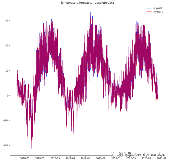
使用训练好的模型,我们可以预测值并将其与原始值进行比较。

中位数绝对误差为0.34摄氏度,平均值为0.48摄氏度。
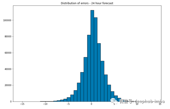
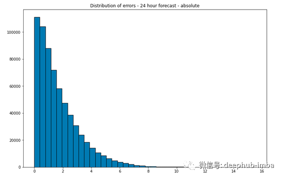
要预测提前24小时,唯一需要做的就是更改超参数。具体来说,是n_ahead变量。该模型将尝试使用之前(一周)的168小时来预测接下来的24小时值。
# Number of lags (hours back) to use for models
lag = 168

# Steps ahead to forecast
n_ahead = 24

# Share of obs in testing
test_share = 0.1

# Epochs for training
epochs = 20

# Batch size
batch_size = 512

# Learning rate
lr = 0.001

# Number of neurons in LSTM layer
n_layer = 10

# Creating the X and Y for training
X, Y = create_X_Y(ts_s.values, lag=lag, n_ahead=n_ahead)n_ft = X.shape[2]Xtrain, Ytrain = X[0:int(X.shape[0] * (1 - test_share))], Y[0:int(X.shape[0] * (1 - test_share))]Xval, Yval = X[int(X.shape[0] * (1 - test_share)):], Y[int(X.shape[0] * (1 - test_share)):]

# Creating the model object
model = NNMultistepModel(
    X=Xtrain,
    Y=Ytrain,
    n_outputs=n_ahead,
    n_lag=lag,
    n_ft=n_ft,
    n_layer=n_layer,
    batch=batch_size,
    epochs=epochs,
    lr=lr,
    Xval=Xval,
    Yval=Yval,
)# Training the model
history = model.train()

检查一些随机的24小时区间:
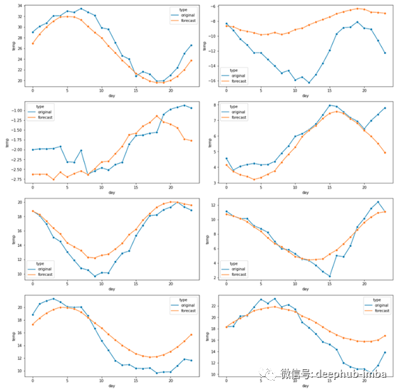
有些24小时序列似乎彼此接近,而其他序列则不然。
平均绝对误差为1.69 C,中位数为1.27C。
总结,本文介绍了在对时间序列数据进行建模和预测时使用的简单管道示例:
读取,清理和扩充输入数据
为滞后和n步选择超参数
为深度学习模型选择超参数
初始化NNMultistepModel()类
拟合模型
预测未来n_steps
最后本文的完整代码:https://github.com/Eligijus112/Vilnius-weather-LSTM
作者:Eligijus Bujokas
deephub翻译组