
SplaTAM全称是《SplaTAM: Splat, Track & Map 3D Gaussians for Dense RGB-D SLAM》,是第一个(也是目前唯一一个)开源的用3D Gaussian Splatting(3DGS)来做SLAM的工作。
在下面博客中,已经对3DGS进行了调研与学习。其中也包含了SplaTAM算法的基本介绍。
学习笔记之——3D Gaussian Splatting及其在SLAM与自动驾驶上的应用调研-CSDN博客文章浏览阅读1.2k次,点赞25次,收藏24次。论文主页3D Gaussian Splatting是最近NeRF方面的突破性工作,它的特点在于重建质量高的情况下还能接入传统光栅化,优化速度也快(能够在较少的训练时间,实现SOTA级别的NeRF的实时渲染效果,且可以以 1080p 分辨率进行高质量的实时(≥ 30 fps)新视图合成)。开山之作就是论文“3D Gaussian Splatting for Real-Time Radiance Field Rendering”是2023年SIGGRAPH最佳论文。https://blog.csdn.net/gwplovekimi/article/details/135397265?spm=1001.2014.3001.5501而在下面博客中,也对3DGS的源码进行了学习
学习笔记之——3D Gaussian Splatting源码解读_3dgs运行代码-CSDN博客文章浏览阅读1k次,点赞14次,收藏24次。高斯模型的初始化,初始化过程中加载或定义了各种相关的属性使用的球谐阶数、最大球谐阶数、各种张量(_xyz等)、优化器和其他参数。self.active_sh_degree = 0 #球谐阶数self.max_sh_degree = sh_degree #最大球谐阶数# 存储不同信息的张量(tensor)self._xyz = torch.empty(0) #空间位置self._scaling = torch.empty(0) #椭球的形状尺度。_3dgs运行代码https://blog.csdn.net/gwplovekimi/article/details/135500438?spm=1001.2014.3001.5501本博文对SplaTAM的源码进行学习。原理部分将不再叙述。本博文意在记录本人学习SplaTAM源码时做的学习记录,仅仅供本人学习记录用~
注释代码仓库:
论文主页:SplaTAM: Splat, Track & Map 3D Gaussians for Dense RGB-D SLAM
论文代码:https://github.com/spla-tam/SplaTAM
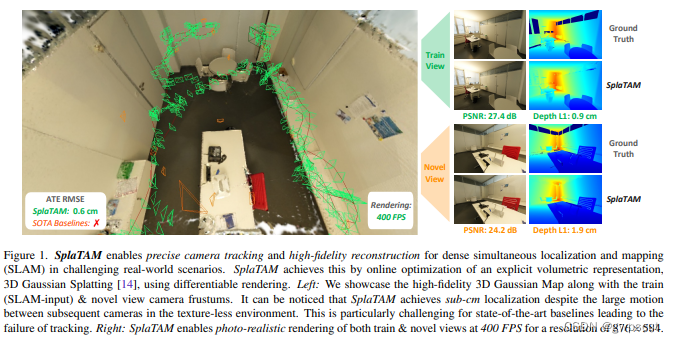
SplaTAM Splat, Track Map 3D Gaussians for Dense RGB-D SLAM
SplaTAM配置
之前博客介绍了3DGS在linux下的配置,基本的设定跟这里很像~
实验笔记之——Gaussian Splatting-CSDN博客文章浏览阅读1.1k次,点赞34次,收藏15次。之前博客对NeRF-SLAM进行了调研学习笔记之——NeRF SLAM(基于神经辐射场的SLAM)-CSDN博客NeRF 所做的任务是 Novel View Synthesis(新视角合成),即在若干已知视角下对场景进行一系列的观测(相机内外参、图像、Pose 等),合成任意新视角下的图像。传统方法中,通常这一任务采用三维重建再渲染的方式实现,NeRF 希望不进行显式的三维重建过程,仅根据内外参直接得到新视角渲染的图像。https://blog.csdn.net/gwplovekimi/article/details/135349210?spm=1001.2014.3001.5501注意SplaTAM需要CUDA>=11.6,而我用的服务器是12.0,满足
首先创建conda环境,并进入
conda create -n splatam python=3.10
conda activate splatam
安装下面依赖
conda install -c "nvidia/label/cuda-11.6.0" cuda-toolkit
conda install pytorch==1.12.1 torchvision==0.13.1 torchaudio==0.12.1 cudatoolkit=11.6 -c pytorch -c conda-forge
然后下载github仓库,并进入相应的路径,运行
git clone https://github.com/spla-tam/SplaTAM --recursive
pip install -r requirements.txt
下载过程有点久~最后却报错如下

再运行一次还是不行。感觉应该是diff-gaussian-rasterization-w-depth.git里面没东西.
先进入/home/gwp/SplaTAM/diff-gaussian-rasterization-w-depth.git,然后进行git下载
git clone https://github.com/JonathonLuiten/diff-gaussian-rasterization-w-depth.git

然后再运行。好像就可以开始build了,希望不要报错。。。。。。

还是不行。尝试下面代码
pip install setuptools wheel
还是不行。尝试改为
pip install diff-gaussian-rasterization-w-depth.git/diff-gaussian-rasterization-w-depth
也不行,改为先删掉这个模块。同时pip install -r requirements.txt注释掉diff-gaussian-rasterization-w-depth.git部分

运行下面的也还是会报错
git clone https://github.com/JonathonLuiten/diff-gaussian-rasterization-w-depth.git

cd diff-gaussian-rasterization-w-depth
python setup.py install
pip install .
感觉还是要回到原本,看看下面这个错误到底是什么
“ERROR: Could not build wheels for diff-gaussian-rasterization, which is required to install pyproject.toml-based projects”
有建议说安装一下Cmake
pip install Cmake
还是不行。。。
(应该这个解决方法最好!其他都不work) 将gcc和g++的版本降低到10
conda install gxx_linux-64=10
终于可以了!(参考:https://github.com/spla-tam/SplaTAM/pull/24)

运行测试
由于是全py,所以不需要编译?只需要下载完依赖就可以用了。接下来是数据集的下载。此处采用TUM-RGBD的数据集
bash bash_scripts/download_tum.sh
见代码内容可知,数据会下载到“data/TUM_RGBD”文件中
mkdir -p data/TUM_RGBD
cd data/TUM_RGBD
wget https://vision.in.tum.de/rgbd/dataset/freiburg1/rgbd_dataset_freiburg1_desk.tgz
tar -xvzf rgbd_dataset_freiburg1_desk.tgz
wget https://cvg.cit.tum.de/rgbd/dataset/freiburg1/rgbd_dataset_freiburg1_desk2.tgz
tar -xvzf rgbd_dataset_freiburg1_desk2.tgz
wget https://cvg.cit.tum.de/rgbd/dataset/freiburg1/rgbd_dataset_freiburg1_room.tgz
tar -xvzf rgbd_dataset_freiburg1_room.tgz
wget https://vision.in.tum.de/rgbd/dataset/freiburg2/rgbd_dataset_freiburg2_xyz.tgz
tar -xvzf rgbd_dataset_freiburg2_xyz.tgz
wget https://vision.in.tum.de/rgbd/dataset/freiburg3/rgbd_dataset_freiburg3_long_office_household.tgz
tar -xvzf rgbd_dataset_freiburg3_long_office_household.tgz

对应文件夹:

然后运行代码(训练指令)如下
tmux new -s splatam   (据说训练时间比较长,还是打开一下tmux吧)
python scripts/splatam.py configs/tum/splatam.py
注意这是对应
freiburg1_desk
场景的。可以打开configs文件看看。其中scene_name就是指定了场景的名字了,而其他的就是参数了
import os
from os.path import join as p_join

primary_device = "cuda:0"

scenes = ["freiburg1_desk", "freiburg1_desk2", "freiburg1_room", "freiburg2_xyz", "freiburg3_long_office_household"]

seed = int(0)
scene_name = scenes[int(0)]

map_every = 1
keyframe_every = 5
mapping_window_size = 20
tracking_iters = 200
mapping_iters = 30
scene_radius_depth_ratio = 2

group_name = "TUM"
run_name = f"{scene_name}_seed{seed}"

config = dict(
    workdir=f"./experiments/{group_name}",
    run_name=run_name,
    seed=seed,
    primary_device=primary_device,
    map_every=map_every, # Mapping every nth frame
    keyframe_every=keyframe_every, # Keyframe every nth frame
    mapping_window_size=mapping_window_size, # Mapping window size
    report_global_progress_every=500, # Report Global Progress every nth frame
    eval_every=500, # Evaluate every nth frame (at end of SLAM)
    scene_radius_depth_ratio=scene_radius_depth_ratio, # Max First Frame Depth to Scene Radius Ratio (For Pruning/Densification)
    mean_sq_dist_method="projective", # ["projective", "knn"] (Type of Mean Squared Distance Calculation for Scale of Gaussians)
    report_iter_progress=False,
    load_checkpoint=False,
    checkpoint_time_idx=0,
    save_checkpoints=False, # Save Checkpoints
    checkpoint_interval=100, # Checkpoint Interval
    use_wandb=True,
    wandb=dict(
        entity="theairlab",
        project="SplaTAM",
        group=group_name,
        name=run_name,
        save_qual=False,
        eval_save_qual=True,
    ),
    data=dict(
        basedir="./data/TUM_RGBD",
        gradslam_data_cfg=f"./configs/data/TUM/{scene_name}.yaml",
        sequence=f"rgbd_dataset_{scene_name}",
        desired_image_height=480,
        desired_image_width=640,
        start=0,
        end=-1,
        stride=1,
        num_frames=-1,
    ),
    tracking=dict(
        use_gt_poses=False, # Use GT Poses for Tracking
        forward_prop=True, # Forward Propagate Poses
        num_iters=tracking_iters,
        use_sil_for_loss=True,
        sil_thres=0.99,
        use_l1=True,
        ignore_outlier_depth_loss=False,
        use_uncertainty_for_loss_mask=False,
        use_uncertainty_for_loss=False,
        use_chamfer=False,
        loss_weights=dict(
            im=0.5,
            depth=1.0,
        ),
        lrs=dict(
            means3D=0.0,
            rgb_colors=0.0,
            unnorm_rotations=0.0,
            logit_opacities=0.0,
            log_scales=0.0,
            cam_unnorm_rots=0.002,
            cam_trans=0.002,
        ),
    ),
    mapping=dict(
        num_iters=mapping_iters,
        add_new_gaussians=True,
        sil_thres=0.5, # For Addition of new Gaussians
        use_l1=True,
        use_sil_for_loss=False,
        ignore_outlier_depth_loss=False,
        use_uncertainty_for_loss_mask=False,
        use_uncertainty_for_loss=False,
        use_chamfer=False,
        loss_weights=dict(
            im=0.5,
            depth=1.0,
        ),
        lrs=dict(
            means3D=0.0001,
            rgb_colors=0.0025,
            unnorm_rotations=0.001,
            logit_opacities=0.05,
            log_scales=0.001,
            cam_unnorm_rots=0.0000,
            cam_trans=0.0000,
        ),
        prune_gaussians=True, # Prune Gaussians during Mapping
        pruning_dict=dict( # Needs to be updated based on the number of mapping iterations
            start_after=0,
            remove_big_after=0,
            stop_after=20,
            prune_every=20,
            removal_opacity_threshold=0.005,
            final_removal_opacity_threshold=0.005,
            reset_opacities=False,
            reset_opacities_every=500, # Doesn't consider iter 0
        ),
        use_gaussian_splatting_densification=False, # Use Gaussian Splatting-based Densification during Mapping
        densify_dict=dict( # Needs to be updated based on the number of mapping iterations
            start_after=500,
            remove_big_after=3000,
            stop_after=5000,
            densify_every=100,
            grad_thresh=0.0002,
            num_to_split_into=2,
            removal_opacity_threshold=0.005,
            final_removal_opacity_threshold=0.005,
            reset_opacities_every=3000, # Doesn't consider iter 0
        ),
    ),
    viz=dict(
        render_mode='color', # ['color', 'depth' or 'centers']
        offset_first_viz_cam=True, # Offsets the view camera back by 0.5 units along the view direction (For Final Recon Viz)
        show_sil=False, # Show Silhouette instead of RGB
        visualize_cams=True, # Visualize Camera Frustums and Trajectory
        viz_w=600, viz_h=340,
        viz_near=0.01, viz_far=100.0,
        view_scale=2,
        viz_fps=5, # FPS for Online Recon Viz
        enter_interactive_post_online=False, # Enter Interactive Mode after Online Recon Viz
    ),
)
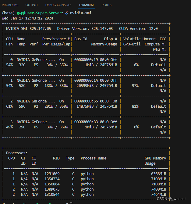
运行成功后,如下所示

同时会创建一个新的文档:

这里很奇怪需要创建账户。。。


但如果旋转了不可视化结果,好像就没办法看了,还是选为1可视化一下
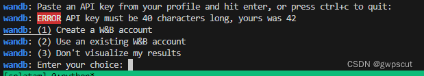
需要40个字节???
1111111111111111111111111111111111111111

好像还是不行。。。
直接把 configs/tum/splatam.py 文件里的 use_wandb = True 改成了 False 就 OK啦。
训练完后,运行下面指令来可视化SplaTAM的重建结果(用MobaXterm)
python viz_scripts/final_recon.py configs/tum/splatam.py
而如果需要看实时的训练效果,则用下面的命令
python viz_scripts/online_recon.py configs/tum/splatam.py
但是却报没有这个文件

原来这个online只是说跑完之后把跑过的按时间跑一遍,所以只能等它跑完了。。。。

大概30分钟左右就可以训练完
下面看看视频效果(可视化训练的过程~看效果好像是把每一次的迭代都分别可视化了,过一会就会重新加载地图模型?但确实好像随着每次代数的增加,要好一些)
SplaTAM Testing using TUM-Dataset freiburg1
由于时间关系就不把全部可视化了,看看全局建模的效果则如下面视频所示(这个UI做得有点差。。。控制得也很不好)
SplaTAM Testing using TUM-Dataset freiburg1
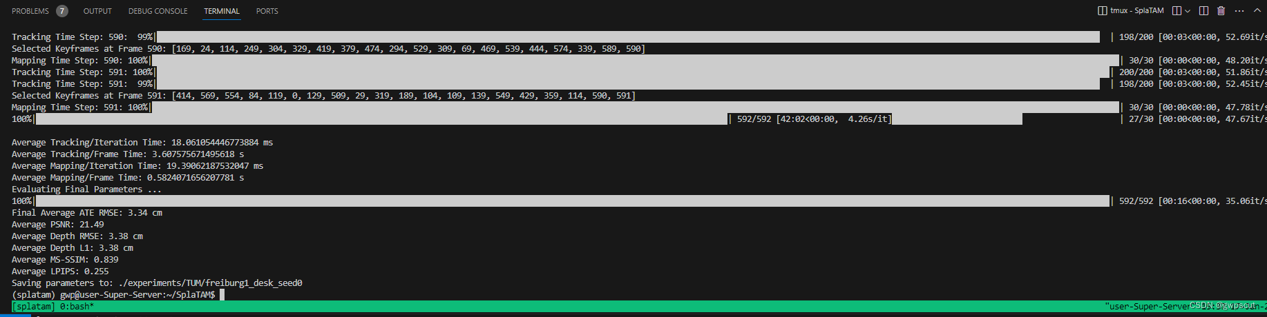
感觉这个效果也一般般,PSNR也是比较差的,当然deth恢复的精度是3.38cm以及定位精度是3.34这个结果还是不错的

更多基于TUM数据集的测试请见博客
实验笔记之——基于TUM-RGBD数据集的SplaTAM测试-CSDN博客文章浏览阅读293次,点赞5次,收藏7次。后面有时间再试试用手机实测来看看吧,不过目前看来用数据集测试的效果都比较差,实时性也很一般,比如rgbd_dataset_freiburg1_desk序列都训练30多分钟了,PSNR还只有21左右,应该3DGS性能不至于这样,可能是因为一些参数的设置包括剪枝等等的操作吧感觉还是有比较大可以研究的空间https://blog.csdn.net/gwplovekimi/article/details/135671402?spm=1001.2014.3001.5501至于在线运行,应该是用iphone就可以了,此处就不进行测试了,还是学习一下源码比较实在~
在下面的源码学习过程中,尽可能的按着思路一个一个代码捋顺,但是由于代码量还是不少,只能将大部分的流程直接写到代码的注释中。
代码解读
从上面介绍可知,直接运行整个程序的代码是Splatam.py,其中后面的py是config,那么前面的就是主程序入口了~
python scripts/splatam.py configs/tum/splatam.py
首先进入main函数
if __name__ == "__main__": # 表示以下的代码块将在脚本作为主程序运行时执行,而不是被导入到其他模块中时执行。
    parser = argparse.ArgumentParser() #创建一个命令行解析器,该解析器将帮助您从命令行接收参数。

    parser.add_argument("experiment", type=str, help="Path to experiment file") #添加一个名为 "experiment" 的命令行参数,它是一个字符串类型,用于指定实验文件的路径。(对应就是config文件内的)

    args = parser.parse_args() #解析命令行参数,将其存储在 args 变量中。

    #使用 SourceFileLoader 加载指定路径的实验文件,并将其作为模块加载到 experiment 变量中。
    experiment = SourceFileLoader(
        os.path.basename(args.experiment), args.experiment
    ).load_module()

    # Set Experiment Seed
    seed_everything(seed=experiment.config['seed']) #设置实验的随机数种子,种子值来自实验配置文件中的 'seed' 字段。

    # Create Results Directory and Copy Config
    # 创建结果目录并复制配置文件:
    results_dir = os.path.join(
        experiment.config["workdir"], experiment.config["run_name"] #存储了实验结果的目录路径,由实验配置文件中的 "workdir" 和 "run_name" 字段组成。
    )
    if not experiment.config['load_checkpoint']: #检查是否需要加载检查点,如果不需要,则执行以下操作:
        os.makedirs(results_dir, exist_ok=True)
        shutil.copy(args.experiment, os.path.join(results_dir, "config.py")) #复制实验配置文件到结果目录下的 "config.py"。

    rgbd_slam(experiment.config) #调用函数rgbd_slam并传递配置文件作为参数
那么接下来就是看主要的运行函数rgbd_slam了。在下面代码之前应该运行的都是一下初始、加载参数等操作。函数的主要功能包括:
- 打印配置信息。
- 创建输出目录。
- 初始化WandB(可选)。
- 加载设备和数据集。
- 迭代处理RGB-D帧,进行跟踪(Tracking)和建图(Mapping)。
- 保存关键帧信息和参数。
- 最后,评估最终的SLAM参数。
    # Iterate over Scan (迭代扫描,迭代处理RGB-D帧,进行跟踪(Tracking)和建图(Mapping))
    for time_idx in tqdm(range(checkpoint_time_idx, num_frames)): #通过循环迭代处理 RGB-D 帧,循环的起始索引是 checkpoint_time_idx(也就是是否从某帧开始,一般都是0开始),终止索引是 num_frames。
        # Load RGBD frames incrementally instead of all frames
        color, depth, _, gt_pose = dataset[time_idx] #从数据集 dataset 中加载 RGB-D 帧的颜色、深度、姿态等信息。
        # Process poses
        gt_w2c = torch.linalg.inv(gt_pose)#对姿态信息进行处理,计算pose的逆,也就是世界到相机的变换矩阵 gt_w2c。

        # Process RGB-D Data
        # 使用了PyTorch中的permute函数,将颜色数据的维度进行重新排列。
        # 在这里,color是一个张量(tensor),通过permute(2, 0, 1)操作,将原始颜色数据的维度顺序从 (height, width, channels) 调整为 (channels, height, width)。
        color = color.permute(2, 0, 1) / 255 #将颜色归一化,归一化到0~1范围
        depth = depth.permute(2, 0, 1)

        # 将当前帧的pose gt_w2c 添加到列表 gt_w2c_all_frames 中。
        gt_w2c_all_frames.append(gt_w2c)
        curr_gt_w2c = gt_w2c_all_frames
        # Optimize only current time step for tracking
        iter_time_idx = time_idx

        # Initialize Mapping Data for selected frame
        # 初始化当前帧的数据 curr_data 包括相机参数、颜色数据、深度数据等。
        curr_data = {'cam': cam, 'im': color, 'depth': depth, 'id': iter_time_idx, 'intrinsics': intrinsics,
                     'w2c': first_frame_w2c, 'iter_gt_w2c_list': curr_gt_w2c}

        # Initialize Data for Tracking(根据配置,初始化跟踪数据 tracking_curr_data。)
        if seperate_tracking_res:
            tracking_color, tracking_depth, _, _ = tracking_dataset[time_idx]
            tracking_color = tracking_color.permute(2, 0, 1) / 255
            tracking_depth = tracking_depth.permute(2, 0, 1)
            tracking_curr_data = {'cam': tracking_cam, 'im': tracking_color, 'depth': tracking_depth, 'id': iter_time_idx,
                                  'intrinsics': tracking_intrinsics, 'w2c': first_frame_w2c, 'iter_gt_w2c_list': curr_gt_w2c}
        else:
            tracking_curr_data = curr_data #初始化跟踪数据

        # Optimization Iterations(设置建图迭代次数)
        num_iters_mapping = config['mapping']['num_iters']

        # Initialize the camera pose for the current frame
        if time_idx > 0: #如果当前帧索引大于 0,则初始化相机姿态参数。
            params = initialize_camera_pose(params, time_idx, forward_prop=config['tracking']['forward_prop']) #参数文件中,forward_prop是true

        # Tracking (进入跟踪阶段,根据当前帧进行优化迭代,包括重置优化器、学习率、迭代过程中的损失计算和优化器更新等。)
        tracking_start_time = time.time()
        if time_idx > 0 and not config['tracking']['use_gt_poses']:
           !一系列操作!

        # Densification & KeyFrame-based Mapping
        # 进入建图阶段,包括密集化和基于关键帧的建图。
        if time_idx == 0 or (time_idx+1) % config['map_every'] == 0:
            !一系列操作!

        # Add frame to keyframe list(将当前帧加入关键帧列表,同时根据配置进行定期的保存检查点。)
        if ((time_idx == 0) or ((time_idx+1) % config['keyframe_every'] == 0) or \
                    (time_idx == num_frames-2)) and (not torch.isinf(curr_gt_w2c[-1]).any()) and (not torch.isnan(curr_gt_w2c[-1]).any()):
            with torch.no_grad():
                # Get the current estimated rotation & translation
                curr_cam_rot = F.normalize(params['cam_unnorm_rots'][..., time_idx].detach())
                curr_cam_tran = params['cam_trans'][..., time_idx].detach()
                curr_w2c = torch.eye(4).cuda().float()
                curr_w2c[:3, :3] = build_rotation(curr_cam_rot)
                curr_w2c[:3, 3] = curr_cam_tran
                # Initialize Keyframe Info
                curr_keyframe = {'id': time_idx, 'est_w2c': curr_w2c, 'color': color, 'depth': depth}
                # Add to keyframe list
                keyframe_list.append(curr_keyframe)
                keyframe_time_indices.append(time_idx)

        # Checkpoint every iteration
        if time_idx % config["checkpoint_interval"] == 0 and config['save_checkpoints']:
            ckpt_output_dir = os.path.join(config["workdir"], config["run_name"])
            save_params_ckpt(params, ckpt_output_dir, time_idx)
            np.save(os.path.join(ckpt_output_dir, f"keyframe_time_indices{time_idx}.npy"), np.array(keyframe_time_indices))

        # Increment WandB Time Step
        if config['use_wandb']: #如果使用 WandB(Weights & Biases),则更新 WandB 的时间步数。
            wandb_time_step += 1

        # 清理 GPU 内存。
        torch.cuda.empty_cache()
而这部分代码之后则是一系列结果的输出,所以关键的tracking部分与mapping部分就是这段代码处理的。由于这段代码有点长。下面拆分为tracking与mapping。但在此之前,先看看如何初始化tracking pose与mapping的高斯点的
初始化tracking pose
        # Initialize the camera pose for the current frame
        if time_idx > 0: #如果当前帧索引大于 0,则初始化相机姿态参数。
            params = initialize_camera_pose(params, time_idx, forward_prop=config['tracking']['forward_prop']) #参数文件中,forward_prop是true
关于初始化相机的位姿initialize_camera_pose,解读如下
# 用于初始化相机姿态的函数
# 根据当前时间初始化相机的旋转和平移参数。(根据前两帧对当前帧的初始pose进行预测)
def initialize_camera_pose(params, curr_time_idx, forward_prop): #参数文件中,forward_prop是true
    with torch.no_grad(): #此用来确保在这个上下文中没有梯度计算。
        if curr_time_idx > 1 and forward_prop: #检查当前时间步 curr_time_idx 是否大于 1,以及是否使用了向前传播
            # Initialize the camera pose for the current frame based on a constant velocity model
            # 使用常速度模型初始化相机姿态。
            # Rotation(通过前两帧的旋转计算出当前帧的新旋转。)
            prev_rot1 = F.normalize(params['cam_unnorm_rots'][..., curr_time_idx-1].detach())
            prev_rot2 = F.normalize(params['cam_unnorm_rots'][..., curr_time_idx-2].detach())
            new_rot = F.normalize(prev_rot1 + (prev_rot1 - prev_rot2))
            params['cam_unnorm_rots'][..., curr_time_idx] = new_rot.detach()

            # Translation(通过前两帧的平移计算出当前帧的新平移。)
            prev_tran1 = params['cam_trans'][..., curr_time_idx-1].detach()
            prev_tran2 = params['cam_trans'][..., curr_time_idx-2].detach()
            new_tran = prev_tran1 + (prev_tran1 - prev_tran2)
            params['cam_trans'][..., curr_time_idx] = new_tran.detach()
        else: #如果条件不满足,则直接复制前一帧的相机姿态到当前帧。这是为了处理初始化的特殊情况,确保在开始时有初始姿态。
            # Initialize the camera pose for the current frame
            params['cam_unnorm_rots'][..., curr_time_idx] = params['cam_unnorm_rots'][..., curr_time_idx-1].detach()
            params['cam_trans'][..., curr_time_idx] = params['cam_trans'][..., curr_time_idx-1].detach()

    return params
总体上,这个函数的作用是为当前帧初始化相机的旋转和平移参数。如果使用了向前传播,它会根据前两帧的信息使用常速度模型进行初始化;否则,直接复制前一帧的姿态。这样的初始化对于建立初始相机姿态是一种常见的方法。
也就是需要预测获得当前帧的初始位姿(作为优化的初值),然后再通过优化来进一步提升这个结果。
初始化mapping(初始化3D高斯点云)
除了初始化位置以外,初始化高斯点云也同样的很重要,见如下代码
                # Add new Gaussians to the scene based on the Silhouette(轮廓,剪影)
                # 高斯分布密集化:
                # 调用 add_new_gaussians 函数,该函数接受当前模型参数 params、变量 variables、密集化数据 densify_curr_data,以及一些配置参数,如阈值、时间索引等。
                # 在 add_new_gaussians 函数中,根据输入的深度图,通过阈值 config['mapping']['sil_thres'] 生成一个Silhouette掩码,然后在场景中添加新的高斯分布。这些高斯分布代表了场景中的新结构。
                params, variables = add_new_gaussians(params, variables, densify_curr_data,
                                                      config['mapping']['sil_thres'], time_idx,
                                                      config['mean_sq_dist_method'])
其中,对于add_new_gaussians函数,下面对详细解读,但此处我们先看看第一帧的时候它会怎么初始化高斯分布
        # 初始化新的高斯分布参数:
        # 利用新的点云和平均平方距离,调用 initialize_new_params 函数生成新的高斯分布参数 new_params。
        new_params = initialize_new_params(new_pt_cld, mean3_sq_dist)
        # 将新的高斯分布参数添加到原有参数中:
        for k, v in new_params.items(): #对于每个键值对 (k, v),其中 k 是高斯分布参数的键,v 是对应的值,在 params 中将其与新参数 v 拼接,并转换为可梯度的 torch.nn.Parameter 对象。
            params[k] = torch.nn.Parameter(torch.cat((params[k], v), dim=0).requires_grad_(True))
        # (更新相关的统计信息)初始化一些统计信息,如梯度累积、分母、最大2D半径等。
        num_pts = params['means3D'].shape[0]
        variables['means2D_gradient_accum'] = torch.zeros(num_pts, device="cuda").float()
        variables['denom'] = torch.zeros(num_pts, device="cuda").float()
        variables['max_2D_radius'] = torch.zeros(num_pts, device="cuda").float()
        # (更新时间步信息)将新的点云对应的时间步信息 new_timestep(都是当前帧的时间步)拼接到原有的时间步信息中。
        new_timestep = time_idx*torch.ones(new_pt_cld.shape[0],device="cuda").float()
        variables['timestep'] = torch.cat((variables['timestep'],new_timestep),dim=0)
其中的函数为
# 初始化新的高斯分布参数
# mean3_sq_dist:新点云的均方距离,用于初始化高斯分布的尺度参数。
def initialize_new_params(new_pt_cld, mean3_sq_dist):
    num_pts = new_pt_cld.shape[0] #点云
    means3D = new_pt_cld[:, :3] # [num_gaussians, 3] #点云对应的位置信息xyz
    unnorm_rots = np.tile([1, 0, 0, 0], (num_pts, 1)) # [num_gaussians, 3]  高斯球的旋转,四元数的未归一化旋转表示,暗示高斯分布没有旋转。
    logit_opacities = torch.zeros((num_pts, 1), dtype=torch.float, device="cuda") #透明度,初始化为0
    params = {
        'means3D': means3D,
        'rgb_colors': new_pt_cld[:, 3:6],
        'unnorm_rotations': unnorm_rots,
        'logit_opacities': logit_opacities,
        'log_scales': torch.tile(torch.log(torch.sqrt(mean3_sq_dist))[..., None], (1, 1)),
    }
    # 构建参数字典 params:params 包含了高斯分布的均值 means3D、颜色 rgb_colors、未归一化旋转 unnorm_rotations、不透明度的对数 logit_opacities 以及尺度的对数 log_scales。
    for k, v in params.items(): #遍历 params 字典,将其值转换为 torch.Tensor 或 torch.nn.Parameter 类型。
        # Check if value is already a torch tensor
        if not isinstance(v, torch.Tensor):
            params[k] = torch.nn.Parameter(torch.tensor(v).cuda().float().contiguous().requires_grad_(True))
        else:
            params[k] = torch.nn.Parameter(v.cuda().float().contiguous().requires_grad_(True))

    return params #返回初始化后的高斯分布参数字典。
那么问题又来了,如何获得这些点云new_pt_cld以及mean3_sq_dist(初始化的高斯尺度)呢?从代码中可以看到是来自于下面的函数
        # 获取新的点云和平均平方距离:
        #利用 get_pointcloud 函数,传入当前帧的图像、深度图、内参、变换矩阵和非存在掩码,生成新的点云 new_pt_cld。同时计算这些新点云到已存在高斯分布的平均平方距离 mean3_sq_dist。
        new_pt_cld, mean3_sq_dist = get_pointcloud(curr_data['im'], curr_data['depth'], curr_data['intrinsics'],
                                    curr_w2c, mask=non_presence_mask, compute_mean_sq_dist=True,
                                    mean_sq_dist_method=mean_sq_dist_method) #参数文件中定义mean_sq_dist_method为projective
对于get_pointcloud函数,其目的就是从给定的颜色图像、深度图像、相机内参和相机到世界坐标系的变换矩阵中获取点云。解读如下
# 从给定的颜色图像、深度图像、相机内参和相机到世界坐标系的变换矩阵中获取点云。
# 输入参数:
# color:RGB颜色图像,形状为 (C, H, W),表示通道数、高度和宽度。
# depth:深度图像,形状为 (1, H, W),只使用深度信息的第一个通道。
# intrinsics:相机内参矩阵,形状为 (3, 3)。
# w2c:相机到世界坐标系的变换矩阵,形状为 (4, 4)。
# transform_pts:一个布尔值,指示是否对点进行坐标变换,默认为 True。
# mask:可选的掩码,形状为 (H * W,),用于选择特定的点云点。
# compute_mean_sq_dist:一个布尔值,指示是否计算均方距离,默认为 False。
# mean_sq_dist_method:均方距离计算方法,目前仅支持 "projective"。
def get_pointcloud(color, depth, intrinsics, w2c, transform_pts=True,
                   mask=None, compute_mean_sq_dist=False, mean_sq_dist_method="projective"):

    # 从颜色图像中提取宽度和高度,并计算相机内参的各个分量。
    width, height = color.shape[2], color.shape[1]
    CX = intrinsics[0][2]
    CY = intrinsics[1][2]
    FX = intrinsics[0][0]
    FY = intrinsics[1][1]

    # Compute indices of pixels
    # 计算像素坐标和深度信息:

    # 利用网格生成像素坐标 xx 和 yy。
    x_grid, y_grid = torch.meshgrid(torch.arange(width).cuda().float(),
                                    torch.arange(height).cuda().float(),
                                    indexing='xy')
    xx = (x_grid - CX)/FX
    yy = (y_grid - CY)/FY
    xx = xx.reshape(-1)
    yy = yy.reshape(-1)
    # 计算深度信息 depth_z。
    depth_z = depth[0].reshape(-1)

    # Initialize point cloud
    # 初始化相机坐标系下的点云
    pts_cam = torch.stack((xx * depth_z, yy * depth_z, depth_z), dim=-1) #利用像素坐标和深度信息初始化相机坐标系下的点云

    # 如果 transform_pts 为 True(默认为true且没有传入参数),则进行坐标变换,将点云从相机坐标系变换到世界坐标系。
    if transform_pts:
        pix_ones = torch.ones(height * width, 1).cuda().float()
        pts4 = torch.cat((pts_cam, pix_ones), dim=1)
        c2w = torch.inverse(w2c)
        pts = (c2w @ pts4.T).T[:, :3]
    else:
        pts = pts_cam

    # Compute mean squared distance for initializing the scale of the Gaussians
    # 根据指定的方法计算均方距离。
    if compute_mean_sq_dist:
        if mean_sq_dist_method == "projective":
            # Projective Geometry (this is fast, farther -> larger radius)
            scale_gaussian = depth_z / ((FX + FY)/2)
            mean3_sq_dist = scale_gaussian**2
        else:
            raise ValueError(f"Unknown mean_sq_dist_method {mean_sq_dist_method}")

    # Colorize point cloud
    # 将点云与颜色信息结合,形成彩色的点云。
    cols = torch.permute(color, (1, 2, 0)).reshape(-1, 3) # (C, H, W) -> (H, W, C) -> (H * W, C)
    point_cld = torch.cat((pts, cols), -1)

    # Select points based on mask
    # 如果提供了掩码 mask,则基于掩码选择特定的点
    if mask is not None:
        point_cld = point_cld[mask]
        if compute_mean_sq_dist:
            mean3_sq_dist = mean3_sq_dist[mask]

    if compute_mean_sq_dist:
        return point_cld, mean3_sq_dist
    else:
        return point_cld
好了,那么这里其实还是在看add_new_gaussians里面的函数,总觉得有点怪(这应该只是每一轮怎么初始化高斯点云)。全局再看看,发现还有一个函数是initialize_first_timestep这个函数才是真正最开始的从第一帧的时候来初始化的,下面看看它是怎么调用get_pointcloud的。
# 这段代码的目的是在初始化时间步骤时设置相机和场景参数,并获取初始点云。
    # 输入参数:
    # dataset:包含RGB-D数据和相机参数的数据集。
    # num_frames:时间步骤数。
    # scene_radius_depth_ratio:用于初始化场景半径的深度比率。
    # mean_sq_dist_method:均方距离计算方法。
    # densify_dataset:可选的用于密集化的数据集。
def initialize_first_timestep(dataset, num_frames, scene_radius_depth_ratio, mean_sq_dist_method, densify_dataset=None):

    # Get RGB-D Data & Camera Parameters
    # 从数据集中获取第一帧RGB-D数据(颜色、深度)、相机内参和相机姿态。
    color, depth, intrinsics, pose = dataset[0]

    # Process RGB-D Data
    # 将颜色数据调整为PyTorch的形状和范围。
    color = color.permute(2, 0, 1) / 255 # (H, W, C) -> (C, H, W)
    # 调整深度数据的形状。
    depth = depth.permute(2, 0, 1) # (H, W, C) -> (C, H, W)

    # Process Camera Parameters
    # 提取相机内参并计算相机到世界坐标系的逆矩阵。
    intrinsics = intrinsics[:3, :3]
    w2c = torch.linalg.inv(pose)

    # Setup Camera
    # 使用提取的相机参数设置相机。
    cam = setup_camera(color.shape[2], color.shape[1], intrinsics.cpu().numpy(), w2c.detach().cpu().numpy())

    if densify_dataset is not None: #如果提供了密集化数据集,获取第一帧RGB-D数据和相机内参,并进行相应的处理。
        # Get Densification RGB-D Data & Camera Parameters
        color, depth, densify_intrinsics, _ = densify_dataset[0]
        color = color.permute(2, 0, 1) / 255 # (H, W, C) -> (C, H, W)
        depth = depth.permute(2, 0, 1) # (H, W, C) -> (C, H, W)
        densify_intrinsics = densify_intrinsics[:3, :3]
        densify_cam = setup_camera(color.shape[2], color.shape[1], densify_intrinsics.cpu().numpy(), w2c.detach().cpu().numpy())
    else:
        densify_intrinsics = intrinsics

    # Get Initial Point Cloud (PyTorch CUDA Tensor)
    mask = (depth > 0) # Mask out invalid depth values
    mask = mask.reshape(-1)
    # 根据颜色、深度、相机内参、相机到世界坐标系的逆矩阵等信息,使用 get_pointcloud 函数获取初始点云。
    # 通过 mask 过滤掉无效深度值。
    init_pt_cld, mean3_sq_dist = get_pointcloud(color, depth, densify_intrinsics, w2c,
                                                mask=mask, compute_mean_sq_dist=True,
                                                mean_sq_dist_method=mean_sq_dist_method)

    # Initialize Parameters
    # 利用初始点云和其他信息,使用 initialize_params 函数初始化模型参数和变量。
    params, variables = initialize_params(init_pt_cld, num_frames, mean3_sq_dist)

    # Initialize an estimate of scene radius for Gaussian-Splatting Densification
    # 估计场景半径,用于后续的高斯光斑密集化。
    variables['scene_radius'] = torch.max(depth)/scene_radius_depth_ratio

    if densify_dataset is not None:
        return params, variables, intrinsics, w2c, cam, densify_intrinsics, densify_cam
    else:
        return params, variables, intrinsics, w2c, cam
其实跟add_new_gaussians里面的是类似的,也都是用所有的图像(彩色与深度)信息来初始化高斯点云~
接下来单独看看tracking部分
Tracking
#################### Tracking (进入跟踪阶段,根据当前帧进行优化迭代,包括重置优化器、学习率、迭代过程中的损失计算和优化器更新等。)
        tracking_start_time = time.time() #记录跟踪阶段的开始时间,用于计时
        # 判断是否采用真值的pose
        if time_idx > 0 and not config['tracking']['use_gt_poses']: #如果当前时间步 time_idx 大于 0 且不使用真实姿态
            # Reset Optimizer & Learning Rates for tracking(重置优化器和学习率,这通常是为了跟踪阶段使用不同的优化设置。)
            optimizer = initialize_optimizer(params, config['tracking']['lrs'], tracking=True)

            # Keep Track of Best Candidate Rotation & Translation(初始化变量 candidate_cam_unnorm_rot 和 candidate_cam_tran 以跟踪最佳的相机旋转和平移。)
            candidate_cam_unnorm_rot = params['cam_unnorm_rots'][..., time_idx].detach().clone()
            candidate_cam_tran = params['cam_trans'][..., time_idx].detach().clone()

            # 初始化变量 current_min_loss 用于跟踪当前迭代中的最小损失。
            current_min_loss = float(1e20)

            # Tracking Optimization(开始进行tracking的优化)
            iter = 0 #设置迭代次数初始值为 0。
            do_continue_slam = False #是否进行运行,用于判断是否满足终止的条件
            num_iters_tracking = config['tracking']['num_iters'] #定义的跟踪迭代次数,参数文件中为200
            progress_bar = tqdm(range(num_iters_tracking), desc=f"Tracking Time Step: {time_idx}") #使用 tqdm 创建一个进度条,显示当前跟踪迭代的进度
            while True:
                iter_start_time = time.time() #记录迭代开始的时间,用于计算迭代的运行时间。

                # Loss for current frame
                # 计算当前帧的损失(loss)
                loss, variables, losses = get_loss(params, tracking_curr_data, variables, iter_time_idx, config['tracking']['loss_weights'],
                                                   config['tracking']['use_sil_for_loss'], config['tracking']['sil_thres'],
                                                   config['tracking']['use_l1'], config['tracking']['ignore_outlier_depth_loss'], tracking=True,
                                                   plot_dir=eval_dir, visualize_tracking_loss=config['tracking']['visualize_tracking_loss'],
                                                   tracking_iteration=iter)

                # 检查是否使用 Weights and Biases(W&B)进行记录和可视化。
                if config['use_wandb']:
                    # Report Loss
                    wandb_tracking_step = report_loss(losses, wandb_run, wandb_tracking_step, tracking=True)

                # Backprop(将loss进行反向传播。计算梯度)
                loss.backward()

                # Optimizer Update(更新优化器。根据计算的梯度更新模型参数。)
                optimizer.step()
                optimizer.zero_grad(set_to_none=True) #清零梯度,以便下一次迭代重新计算梯度。

                with torch.no_grad(): #进入没有梯度的上下文,下面的操作不会影响梯度计算。
                    # Save the best candidate rotation & translation(记录最小损失对应的相机旋转和平移。)
                    if loss < current_min_loss: #如果当前损失小于 current_min_loss,更新最小损失对应的相机旋转和平移。
                        current_min_loss = loss
                        candidate_cam_unnorm_rot = params['cam_unnorm_rots'][..., time_idx].detach().clone()
                        candidate_cam_tran = params['cam_trans'][..., time_idx].detach().clone()
                    # Report Progress
                    if config['report_iter_progress']: #如果配置中启用了报告迭代进度 (config['report_iter_progress']),执行报告进度的操作。
                        if config['use_wandb']:
                            report_progress(params, tracking_curr_data, iter+1, progress_bar, iter_time_idx, sil_thres=config['tracking']['sil_thres'], tracking=True,
                                            wandb_run=wandb_run, wandb_step=wandb_tracking_step, wandb_save_qual=config['wandb']['save_qual'])
                        else:
                            report_progress(params, tracking_curr_data, iter+1, progress_bar, iter_time_idx, sil_thres=config['tracking']['sil_thres'], tracking=True)
                    else:
                        progress_bar.update(1)

                # Update the runtime numbers (更新迭代次数和计算迭代的运行时间。)
                iter_end_time = time.time()
                tracking_iter_time_sum += iter_end_time - iter_start_time
                tracking_iter_time_count += 1

                # Check if we should stop tracking(检查是否最大迭代次数,满足终止计算)
                iter += 1
                if iter == num_iters_tracking: #(如果配置中定义的条件满足,则终止跟踪迭代。)
                    if losses['depth'] < config['tracking']['depth_loss_thres'] and config['tracking']['use_depth_loss_thres']:#如果启用了深度损失门限 (config['tracking']['use_depth_loss_thres']) 且深度损失小于门限,则终止迭代。
                        break
                    elif config['tracking']['use_depth_loss_thres'] and not do_continue_slam: #如果启用了深度损失门限且 do_continue_slam为false,则将 do_continue_slam 设置为 True,并增加迭代次数。
                        do_continue_slam = True
                        progress_bar = tqdm(range(num_iters_tracking), desc=f"Tracking Time Step: {time_idx}")
                        num_iters_tracking = 2*num_iters_tracking
                        if config['use_wandb']:
                            wandb_run.log({"Tracking/Extra Tracking Iters Frames": time_idx,
                                        "Tracking/step": wandb_time_step})
                    else:
                        break

            progress_bar.close()
            # Copy over the best candidate rotation & translation
            with torch.no_grad():
                params['cam_unnorm_rots'][..., time_idx] = candidate_cam_unnorm_rot
                params['cam_trans'][..., time_idx] = candidate_cam_tran
        elif time_idx > 0 and config['tracking']['use_gt_poses']: #采用真值的pose来做tracking
            with torch.no_grad(): #进入没有梯度的上下文,下面的操作不会影响梯度计算。(用真值的pose也确实不应该进行梯度的计算)
                # Get the ground truth pose relative to frame 0
                rel_w2c = curr_gt_w2c[-1] #获取当前时间帧的真值姿态相对于第 0 帧的相机到世界坐标系的变换矩阵。
                rel_w2c_rot = rel_w2c[:3, :3].unsqueeze(0).detach() #提取相机旋转矩阵,并在第 0 维度上增加一个维度,转换成形状为 (1, 3, 3) 的张量。
                rel_w2c_rot_quat = matrix_to_quaternion(rel_w2c_rot) #将相机旋转矩阵转换为四元数。
                rel_w2c_tran = rel_w2c[:3, 3].detach() #提取相机平移矩阵。
                # Update the camera parameters
                params['cam_unnorm_rots'][..., time_idx] = rel_w2c_rot_quat #将真值姿态的四元数赋值给相机旋转参数。
                params['cam_trans'][..., time_idx] = rel_w2c_tran #将真值姿态的平移矩阵赋值给相机平移参数(参数用作全局变量了)。
        # Update the runtime numbers
        tracking_end_time = time.time()
        tracking_frame_time_sum += tracking_end_time - tracking_start_time
        tracking_frame_time_count += 1
 #################### ####################
对于tracking中loss的计算,可以看函数get_loss,主要用于在跟踪(tracking)或映射(mapping)过程中评估当前帧的损失。tracking与mapping都是用这个函数
# 主要用于在跟踪(tracking)或映射(mapping)过程中评估当前帧的损失。
# 函数接受一系列输入参数,包括相机参数 params、当前数据 curr_data、一些中间变量 variables、迭代的时间步 iter_time_idx、损失权重 loss_weights、是否使用深度图用于损失计算 use_sil_for_loss、阈值 sil_thres 等等。
def get_loss(params, curr_data, variables, iter_time_idx, loss_weights, use_sil_for_loss,
             sil_thres, use_l1,ignore_outlier_depth_loss, tracking=False,
             mapping=False, do_ba=False, plot_dir=None, visualize_tracking_loss=False, tracking_iteration=None):
    # Initialize Loss Dictionary
    losses = {}

    # 根据输入的参数和当前迭代的时间步,调用 transform_to_frame 函数将世界坐标系中的点转换为相机坐标系中的高斯分布中心点,并考虑是否需要计算梯度。不同的模式(tracking、mapping)会影响对哪些参数计算梯度。
    # transform_to_frame执行了从世界坐标系到相机坐标系的高斯分布中心点的转换操作,同时考虑了是否需要计算梯度。
    # tracking的时候camera pose需要计算梯度,mapping的时候BA优化,则高斯和pose的梯度都要优化,而单纯的mapping则只需要优化高斯的梯度
    if tracking:
        # Get current frame Gaussians, where only the camera pose gets gradient
        transformed_pts = transform_to_frame(params, iter_time_idx,
                                             gaussians_grad=False,
                                             camera_grad=True)
    elif mapping:
        if do_ba:
            # Get current frame Gaussians, where both camera pose and Gaussians get gradient
            transformed_pts = transform_to_frame(params, iter_time_idx,
                                                 gaussians_grad=True,
                                                 camera_grad=True)
        else:
            # Get current frame Gaussians, where only the Gaussians get gradient
            transformed_pts = transform_to_frame(params, iter_time_idx,
                                                 gaussians_grad=True,
                                                 camera_grad=False)
    else:
        # Get current frame Gaussians, where only the Gaussians get gradient
        transformed_pts = transform_to_frame(params, iter_time_idx,
                                             gaussians_grad=True,
                                             camera_grad=False)


    # Initialize Render Variables (初始化一些渲染的变量)
    #将输入的参数 params 转换成一个包含渲染相关变量的字典 rendervar与depth_sil_rendervar
    rendervar = transformed_params2rendervar(params, transformed_pts)
    depth_sil_rendervar = transformed_params2depthplussilhouette(params, curr_data['w2c'],
                                                                 transformed_pts)

    # RGB Rendering
    rendervar['means2D'].retain_grad() #在进行RGB渲染时,保留其梯度信息(means2D)。
    # 使用渲染器 Renderer 对当前帧进行RGB渲染,得到RGB图像 im、半径信息 radius。
    im, radius, _, = Renderer(raster_settings=curr_data['cam'])(**rendervar) #这里的Renderer是import from diff_gaussian_rasterization,也就是高斯光栅化的渲染
    # 将 means2D 的梯度累积到 variables 中,这是为了在颜色渲染过程中进行密集化(densification)。
    variables['means2D'] = rendervar['means2D']  # Gradient only accum from colour render for densification

    # Depth & Silhouette Rendering
    # 使用渲染器 Renderer 对当前帧进行深度和轮廓渲染,得到深度轮廓图 depth_sil。
    depth_sil, _, _, = Renderer(raster_settings=curr_data['cam'])(**depth_sil_rendervar)
    # 从深度轮廓图中提取深度信息 depth,轮廓信息 silhouette,以及深度的平方 depth_sq。
    depth = depth_sil[0, :, :].unsqueeze(0)
    silhouette = depth_sil[1, :, :]
    presence_sil_mask = (silhouette > sil_thres)
    depth_sq = depth_sil[2, :, :].unsqueeze(0)
    # 计算深度的不确定性,即深度平方的差值,然后将其分离出来并进行 detach 操作(不计算梯度)。
    uncertainty = depth_sq - depth**2
    uncertainty = uncertainty.detach()

    # Mask with valid depth values (accounts for outlier depth values)
    # 建一个 nan_mask,用于标记深度和不确定性的有效值,避免处理异常值。
    nan_mask = (~torch.isnan(depth)) & (~torch.isnan(uncertainty))
    if ignore_outlier_depth_loss: #如果开启了 ignore_outlier_depth_loss,则基于深度误差生成一个新的掩码 mask,并且该掩码会剔除深度值异常的区域。
        depth_error = torch.abs(curr_data['depth'] - depth) * (curr_data['depth'] > 0)
        mask = (depth_error < 10*depth_error.median())
        mask = mask & (curr_data['depth'] > 0)
    else: #如果没有开启 ignore_outlier_depth_loss,则直接使用深度大于零的区域作为 mask。
        mask = (curr_data['depth'] > 0)
    mask = mask & nan_mask
    # Mask with presence silhouette mask (accounts for empty space)
    # 如果在跟踪模式下且开启了使用轮廓图进行损失计算 (use_sil_for_loss),则将 mask 与轮廓图的存在性掩码 presence_sil_mask 相与。
    if tracking and use_sil_for_loss:
        mask = mask & presence_sil_mask

    # 至此,生成RGB图像、深度图、并根据需要进行掩码处理,以便后续在计算损失时使用。

    # Depth loss(计算深度的loss)
    if use_l1: #如果使用L1损失 (use_l1),则将 mask 进行 detach 操作,即不计算其梯度。
        mask = mask.detach()
        if tracking: #如果在跟踪模式下 (tracking),计算深度损失 (losses['depth']) 为当前深度图与渲染深度图之间差值的绝对值之和(只考虑掩码内的区域)。
            losses['depth'] = torch.abs(curr_data['depth'] - depth)[mask].sum()
        else: #如果不在跟踪模式下,计算深度损失为当前深度图与渲染深度图之间差值的绝对值的平均值(只考虑掩码内的区域)。上下一模一样
            losses['depth'] = torch.abs(curr_data['depth'] - depth)[mask].mean()

    # RGB Loss(计算RGB的loss)
    # 如果在跟踪模式下 (tracking) 并且使用轮廓图进行损失计算 (use_sil_for_loss) 或者忽略异常深度值 (ignore_outlier_depth_loss),计算RGB损失 (losses['im']) 为当前图像与渲染图像之间差值的绝对值之和(只考虑掩码内的区域)。
    if tracking and (use_sil_for_loss or ignore_outlier_depth_loss):
        color_mask = torch.tile(mask, (3, 1, 1))
        color_mask = color_mask.detach()
        losses['im'] = torch.abs(curr_data['im'] - im)[color_mask].sum()
    elif tracking: #如果在跟踪模式下,但没有使用轮廓图进行损失计算,计算RGB损失为当前图像与渲染图像之间差值的绝对值之和。
        losses['im'] = torch.abs(curr_data['im'] - im).sum()
    else: #如果不在跟踪模式下,计算RGB损失为L1损失和结构相似性损失的加权和,其中 l1_loss_v1 是L1损失的计算函数,calc_ssim 是结构相似性损失的计算函数。
        losses['im'] = 0.8 * l1_loss_v1(im, curr_data['im']) + 0.2 * (1.0 - calc_ssim(im, curr_data['im']))

    # Visualize the Diff Images
    if tracking and visualize_tracking_loss:
        fig, ax = plt.subplots(2, 4, figsize=(12, 6))
        weighted_render_im = im * color_mask
        weighted_im = curr_data['im'] * color_mask
        weighted_render_depth = depth * mask
        weighted_depth = curr_data['depth'] * mask
        diff_rgb = torch.abs(weighted_render_im - weighted_im).mean(dim=0).detach().cpu()
        diff_depth = torch.abs(weighted_render_depth - weighted_depth).mean(dim=0).detach().cpu()
        viz_img = torch.clip(weighted_im.permute(1, 2, 0).detach().cpu(), 0, 1)
        ax[0, 0].imshow(viz_img)
        ax[0, 0].set_title("Weighted GT RGB")
        viz_render_img = torch.clip(weighted_render_im.permute(1, 2, 0).detach().cpu(), 0, 1)
        ax[1, 0].imshow(viz_render_img)
        ax[1, 0].set_title("Weighted Rendered RGB")
        ax[0, 1].imshow(weighted_depth[0].detach().cpu(), cmap="jet", vmin=0, vmax=6)
        ax[0, 1].set_title("Weighted GT Depth")
        ax[1, 1].imshow(weighted_render_depth[0].detach().cpu(), cmap="jet", vmin=0, vmax=6)
        ax[1, 1].set_title("Weighted Rendered Depth")
        ax[0, 2].imshow(diff_rgb, cmap="jet", vmin=0, vmax=0.8)
        ax[0, 2].set_title(f"Diff RGB, Loss: {torch.round(losses['im'])}")
        ax[1, 2].imshow(diff_depth, cmap="jet", vmin=0, vmax=0.8)
        ax[1, 2].set_title(f"Diff Depth, Loss: {torch.round(losses['depth'])}")
        ax[0, 3].imshow(presence_sil_mask.detach().cpu(), cmap="gray")
        ax[0, 3].set_title("Silhouette Mask")
        ax[1, 3].imshow(mask[0].detach().cpu(), cmap="gray")
        ax[1, 3].set_title("Loss Mask")
        # Turn off axis
        for i in range(2):
            for j in range(4):
                ax[i, j].axis('off')
        # Set Title
        fig.suptitle(f"Tracking Iteration: {tracking_iteration}", fontsize=16)
        # Figure Tight Layout
        fig.tight_layout()
        os.makedirs(plot_dir, exist_ok=True)
        plt.savefig(os.path.join(plot_dir, f"tmp.png"), bbox_inches='tight')
        plt.close()
        plot_img = cv2.imread(os.path.join(plot_dir, f"tmp.png"))
        cv2.imshow('Diff Images', plot_img)
        cv2.waitKey(1)
        ## Save Tracking Loss Viz
        # save_plot_dir = os.path.join(plot_dir, f"tracking_%04d" % iter_time_idx)
        # os.makedirs(save_plot_dir, exist_ok=True)
        # plt.savefig(os.path.join(save_plot_dir, f"%04d.png" % tracking_iteration), bbox_inches='tight')
        # plt.close()

    # 下面代码进行了损失的加权和最终的损失值计算
    # 对每个损失项按照其权重进行加权,得到 weighted_losses 字典,其中 k 是损失项的名称,v 是对应的损失值,loss_weights 是各个损失项的权重。
    weighted_losses = {k: v * loss_weights[k] for k, v in losses.items()}
    # 最终损失值 loss 是加权损失项的和。
    loss = sum(weighted_losses.values())

    seen = radius > 0 #创建一个布尔掩码 seen,其中对应的位置为 True 表示在当前迭代中观察到了某个点。
    variables['max_2D_radius'][seen] = torch.max(radius[seen], variables['max_2D_radius'][seen]) #更新 variables['max_2D_radius'] 中已观察到的点的最大半径。
    variables['seen'] = seen #将 seen 存储在 variables 字典中。
    weighted_losses['loss'] = loss #最终,将总损失值存储在 weighted_losses 字典中的 'loss' 键下。

    return loss, variables, weighted_losses
其中的transform_to_frame跳进去看看,解析如下
# 这个函数的目的是将各向同性高斯分布的中心点从世界坐标系转换到相机坐标系中。
def transform_to_frame(params, time_idx, gaussians_grad, camera_grad):
    """
    Function to transform Isotropic Gaussians from world frame to camera frame.

    Args:
        params: dict of parameters 一个包含各种参数的字典
        time_idx: time index to transform to 表示时间索引,用于指定转换到哪一帧。
        gaussians_grad: enable gradients for Gaussians  一个布尔值,表示是否启用高斯分布的梯度。
        camera_grad: enable gradients for camera pose 一个布尔值,表示是否启用相机位姿的梯度。

    Returns:
        transformed_pts: Transformed Centers of Gaussians #返回的高斯中心点的变换
    """
    # Get Frame Camera Pose 获取相机位姿:
    if camera_grad: #如果 camera_grad 为 True,则获取未归一化的相机旋转 cam_rot 和相机平移 cam_tran
        cam_rot = F.normalize(params['cam_unnorm_rots'][..., time_idx])
        cam_tran = params['cam_trans'][..., time_idx]
    else: #否则,使用 .detach() 方法获取它们的副本,确保梯度不会在这里传播。
        cam_rot = F.normalize(params['cam_unnorm_rots'][..., time_idx].detach())
        cam_tran = params['cam_trans'][..., time_idx].detach()
    # 构建相机到世界坐标系的变换矩阵 rel_w2c,其中包含旋转矩阵和平移向量。
    rel_w2c = torch.eye(4).cuda().float()
    rel_w2c[:3, :3] = build_rotation(cam_rot)
    rel_w2c[:3, 3] = cam_tran

    # Get Centers and norm Rots of Gaussians in World Frame 获取世界坐标系下高斯分布中心和归一化旋转:
    if gaussians_grad: #如果 gaussians_grad 为 True,则获取高斯分布的中心点 pts(不使用 .detach(),所以 pts 是原始张量,它可能是需要计算梯度的。)
        pts = params['means3D']
    else:#。否则,使用 .detach() 方法获取其副本(通过使用 .detach() 方法,确保返回的张量是不需要计算梯度的。这可以防止梯度在这个张量上进行传播。)。
        pts = params['means3D'].detach()

    # Transform Centers and Unnorm Rots of Gaussians to Camera Frame 将中心点和未归一化旋转转换到相机坐标系:
    pts_ones = torch.ones(pts.shape[0], 1).cuda().float() #构建形状为 (N, 4) 的矩阵 pts4,其中 N 是中心点数量,通过在中心点矩阵的最后一列添加全为1的列得到。
    # .cuda() 表示将张量移动到GPU上,如果GPU可用的话。
    # .float() 将张量的数据类型转换为浮点型。
    pts4 = torch.cat((pts, pts_ones), dim=1) #使用 torch.cat 函数在第二维度上拼接 pts 和 pts_ones。(结果是一个形状为 (N, 4) 的张量 pts4,其中最后一列全为1,用于表示齐次坐标。)
    transformed_pts = (rel_w2c @ pts4.T).T[:, :3] #利用相机到世界坐标系的变换矩阵 rel_w2c,将这个矩阵应用于 pts4,并提取结果的前三列,得到转换后的中心点 transformed_pts。
    # 将 pts4 转置(.T)后,利用相机到世界坐标系的变换矩阵 rel_w2c 将其应用于高斯分布的中心点。
    # 将结果再次转置,然后取前三列,得到形状为 (N, 3) 的张量 transformed_pts。
    # 这样得到的 transformed_pts 就是高斯分布中心点在相机坐标系中的转换结果,保留了前三个坐标值。

    return transformed_pts #返回转换后的中心点 transformed_pts。
对于tracking部分,高斯的梯度为false,camera pose的梯度变换为true(tracking的时候camera pose需要计算梯度,mapping的时候BA优化,则高斯和pose的梯度都要优化,而单纯的mapping则只需要优化高斯的梯度)
注意:
detach是 PyTorch 中的方法,用于从计算图中分离张量,使其不再与梯度计算相关。在深度学习中,通常使用自动微分机制来计算梯度,但有时我们希望对某些张量进行操作而不影响梯度的计算,这时就可以使用
detach方法。
        transformed_pts = transform_to_frame(params, iter_time_idx,
                                             gaussians_grad=False,
                                             camera_grad=True)
总体而言,这段代码执行了从世界坐标系到相机坐标系的高斯分布中心点的转换操作,同时考虑了是否需要计算梯度。
Tracking处理之后,mapping处理之前,还有下面这么一段,就是用来更新tracking的效果的(代码中较多这些信息,实际上都是不影响主要逻辑的,阅读代码的时候应该先剥离,不然代码就很冗余,难以理顺清晰的脉络)
        # 如果当前帧索引是第一帧或者符合全局报告进度的条件,则报告跟踪进度。
        if time_idx == 0 or (time_idx+1) % config['report_global_progress_every'] == 0: #确定是否需要报告全局进度。条件满足的情况包括当前帧索引是第一帧,或者当前帧索引符合全局报告进度的条件
            try:
                # Report Final Tracking Progress
                progress_bar = tqdm(range(1), desc=f"Tracking Result Time Step: {time_idx}") #创建一个进度条 progress_bar,用于显示当前进度。
                with torch.no_grad(): #调用 report_progress 函数报告跟踪进度。这里的 with torch.no_grad() 确保在这个过程中不会记录梯度信息,因为报告进度通常不需要进行梯度计算。
                    if config['use_wandb']: #如果使用了 WandB(Weights & Biases)工具,会将相关信息记录到 WandB 的运行中,以便进行可视化和追踪。
                        report_progress(params, tracking_curr_data, 1, progress_bar, iter_time_idx, sil_thres=config['tracking']['sil_thres'], tracking=True,
                                        wandb_run=wandb_run, wandb_step=wandb_time_step, wandb_save_qual=config['wandb']['save_qual'], global_logging=True)
                    else:
                        report_progress(params, tracking_curr_data, 1, progress_bar, iter_time_idx, sil_thres=config['tracking']['sil_thres'], tracking=True)
                progress_bar.close()
            except: #如果报告进度出现异常(except 块),会进行异常处理:
                ckpt_output_dir = os.path.join(config["workdir"], config["run_name"])
                save_params_ckpt(params, ckpt_output_dir, time_idx) #将当前模型参数保存到检查点文件,以便后续恢复。
                print('Failed to evaluate trajectory.') #输出一条提示信息,指示评估轨迹失败。
这段代码用于定期报告跟踪的全局进度,并在异常情况下保存当前模型参数的检查点。
Mapping
if time_idx == 0 or (time_idx+1) % config['map_every'] == 0: #如果当前帧索引是第一帧或者满足 config['map_every'] (每多少帧进行mapping一次)条件时
由于mappping部分代码太长了,此处将其分为致密化、添加建图关键帧以及mapping计算(全局ba)三个模块
致密化(Densification)
            # Densification(首先进行密集化)
            if config['mapping']['add_new_gaussians'] and time_idx > 0: #如果开启了 config['mapping']['add_new_gaussians'],并且当前帧索引大于0,则根据当前帧的数据密集化场景中的新高斯分布。
                # Setup Data for Densification
                if seperate_densification_res:
                    # Load RGBD frames incrementally instead of all frames
                    densify_color, densify_depth, _, _ = densify_dataset[time_idx] #从 densify_dataset 中加载RGBD帧的数据
                    # 对RGB和深度数据进行处理,将RGB数据的维度调整为(3, H, W),将RGB数据的范围缩放到[0, 1]。
                    densify_color = densify_color.permute(2, 0, 1) / 255
                    densify_depth = densify_depth.permute(2, 0, 1)
                    # 构建 densify_curr_data 字典,包含了用于密集化的数据,如相机矩阵、RGB图像、深度图、帧索引等信息。
                    densify_curr_data = {'cam': densify_cam, 'im': densify_color, 'depth': densify_depth, 'id': time_idx,
                                 'intrinsics': densify_intrinsics, 'w2c': first_frame_w2c, 'iter_gt_w2c_list': curr_gt_w2c}
                else:
                    densify_curr_data = curr_data #使用当前帧的数据。

                # Add new Gaussians to the scene based on the Silhouette(轮廓,剪影)
                # 高斯分布密集化:
                # 调用 add_new_gaussians 函数,该函数接受当前模型参数 params、变量 variables、密集化数据 densify_curr_data,以及一些配置参数,如阈值、时间索引等。
                # 在 add_new_gaussians 函数中,根据输入的深度图,通过阈值 config['mapping']['sil_thres'] 生成一个Silhouette掩码,然后在场景中添加新的高斯分布。这些高斯分布代表了场景中的新结构。
                params, variables = add_new_gaussians(params, variables, densify_curr_data,
                                                      config['mapping']['sil_thres'], time_idx,
                                                      config['mean_sq_dist_method'])
                # 记录高斯分布数量:
                post_num_pts = params['means3D'].shape[0] #获取密集化后的高斯分布的数量,并将其记录为 post_num_pts。
                if config['use_wandb']: #如果使用了 WandB,则将密集化后的高斯分布数量和当前迭代步数记录到 WandB 中,以便在 WandB 仪表板中进行监控。
                    wandb_run.log({"Mapping/Number of Gaussians": post_num_pts,
                                   "Mapping/step": wandb_time_step})
对于其中的add_new_gaussians函数现了在建图过程中根据当前帧的数据进行高斯分布的密集化,解读如下
# 现了在建图过程中根据当前帧的数据进行高斯分布的密集化,
def add_new_gaussians(params, variables, curr_data, sil_thres, time_idx, mean_sq_dist_method):
    # Silhouette Rendering
    transformed_pts = transform_to_frame(params, time_idx, gaussians_grad=False, camera_grad=False)#将高斯模型转换到frame坐标系下
    depth_sil_rendervar = transformed_params2depthplussilhouette(params, curr_data['w2c'],
                                                                 transformed_pts) #获取深度的渲染变量
    # 通过渲染器 Renderer 得到深度图和轮廓图,其中 depth_sil 包含了深度信息和轮廓信息。
    depth_sil, _, _, = Renderer(raster_settings=curr_data['cam'])(**depth_sil_rendervar)
    silhouette = depth_sil[1, :, :]
    # non_presence_sil_mask代表当前帧中未出现的区域?
    non_presence_sil_mask = (silhouette < sil_thres) #通过设置阈值 sil_thres(输入参数为0.5),创建一个轮廓图的非存在掩码

    # Check for new foreground objects by using GT depth
    # 利用当前深度图和渲染后的深度图,通过 depth_error 计算深度误差,并生成深度非存在掩码 non_presence_depth_mask。
    gt_depth = curr_data['depth'][0, :, :]
    render_depth = depth_sil[0, :, :]
    depth_error = torch.abs(gt_depth - render_depth) * (gt_depth > 0)
    non_presence_depth_mask = (render_depth > gt_depth) * (depth_error > 50*depth_error.median())

    # Determine non-presence mask
    # 将轮廓图非存在掩码和深度非存在掩码合并生成整体的非存在掩码 non_presence_mask。
    non_presence_mask = non_presence_sil_mask | non_presence_depth_mask
    # Flatten mask
    non_presence_mask = non_presence_mask.reshape(-1)

    # Get the new frame Gaussians based on the Silhouette
    # 检测到非存在掩码中有未出现的点时,根据当前帧的数据生成新的高斯分布参数,并将这些参数添加到原有的高斯分布参数中
    if torch.sum(non_presence_mask) > 0:
        # Get the new pointcloud in the world frame
        # 获取当前相机的旋转和平移信息:
        curr_cam_rot = torch.nn.functional.normalize(params['cam_unnorm_rots'][..., time_idx].detach()) #获取当前帧的相机未归一化旋转信息。
        curr_cam_tran = params['cam_trans'][..., time_idx].detach() #对旋转信息进行归一化。
        # 构建当前帧相机到世界坐标系的变换矩阵:
        curr_w2c = torch.eye(4).cuda().float() #创建一个单位矩阵
        # 利用归一化后的旋转信息和当前帧的相机平移信息,更新变换矩阵的旋转和平移部分。
        curr_w2c[:3, :3] = build_rotation(curr_cam_rot)
        curr_w2c[:3, 3] = curr_cam_tran
        # 生成有效深度掩码:
        valid_depth_mask = (curr_data['depth'][0, :, :] > 0) #生成当前帧的有效深度掩码 valid_depth_mask。
        # 更新非存在掩码:
        non_presence_mask = non_presence_mask & valid_depth_mask.reshape(-1) #将 non_presence_mask 和 valid_depth_mask 进行逐元素与操作,得到更新后的非存在掩码。
        # 获取新的点云和平均平方距离:
        #利用 get_pointcloud 函数,传入当前帧的图像、深度图、内参、变换矩阵和非存在掩码,生成新的点云 new_pt_cld。同时计算这些新点云到已存在高斯分布的平均平方距离 mean3_sq_dist。
        new_pt_cld, mean3_sq_dist = get_pointcloud(curr_data['im'], curr_data['depth'], curr_data['intrinsics'],
                                    curr_w2c, mask=non_presence_mask, compute_mean_sq_dist=True,
                                    mean_sq_dist_method=mean_sq_dist_method)
        # 初始化新的高斯分布参数:
        # 利用新的点云和平均平方距离,调用 initialize_new_params 函数生成新的高斯分布参数 new_params。
        new_params = initialize_new_params(new_pt_cld, mean3_sq_dist)
        # 将新的高斯分布参数添加到原有参数中:
        for k, v in new_params.items(): #对于每个键值对 (k, v),其中 k 是高斯分布参数的键,v 是对应的值,在 params 中将其与新参数 v 拼接,并转换为可梯度的 torch.nn.Parameter 对象。
            params[k] = torch.nn.Parameter(torch.cat((params[k], v), dim=0).requires_grad_(True))
        # (更新相关的统计信息)初始化一些统计信息,如梯度累积、分母、最大2D半径等。
        num_pts = params['means3D'].shape[0]
        variables['means2D_gradient_accum'] = torch.zeros(num_pts, device="cuda").float()
        variables['denom'] = torch.zeros(num_pts, device="cuda").float()
        variables['max_2D_radius'] = torch.zeros(num_pts, device="cuda").float()
        # (更新时间步信息)将新的点云对应的时间步信息 new_timestep(都是当前帧的时间步)拼接到原有的时间步信息中。
        new_timestep = time_idx*torch.ones(new_pt_cld.shape[0],device="cuda").float()
        variables['timestep'] = torch.cat((variables['timestep'],new_timestep),dim=0)

    # 将更新后的模型参数 params 和相关的统计信息 variables 返回。
    return params, variables
这段代码的功能是检测未出现的点,生成新的高斯分布参数,并将其添加到原有的高斯分布参数中,以实现对模型的动态更新。
注意代码中的params就是3D 高斯待优化的参数,其定义如下
    params = {
        'means3D': means3D,
        'rgb_colors': new_pt_cld[:, 3:6],
        'unnorm_rotations': unnorm_rots,
        'logit_opacities': logit_opacities,
        'log_scales': torch.tile(torch.log(torch.sqrt(mean3_sq_dist))[..., None], (1, 1)),
    }
选择关键帧
            # 选择用于建图的关键帧
            with torch.no_grad():
                # Get the current estimated rotation & translation
                # 获取当前帧的估计旋转和平移:
                curr_cam_rot = F.normalize(params['cam_unnorm_rots'][..., time_idx].detach()) #获取当前帧的相机未归一化旋转信息。(使用 F.normalize 对旋转信息进行归一化。)
                curr_cam_tran = params['cam_trans'][..., time_idx].detach() #获取当前帧的相机平移信息
                # 构建当前帧相机到世界坐标系的变换矩阵:
                curr_w2c = torch.eye(4).cuda().float() #创建一个单位矩阵
                # 利用归一化后的旋转信息和当前帧的相机平移信息,更新变换矩阵的旋转和平移部分。
                curr_w2c[:3, :3] = build_rotation(curr_cam_rot)
                curr_w2c[:3, 3] = curr_cam_tran
                # Select Keyframes for Mapping (选择关键帧)
                num_keyframes = config['mapping_window_size']-2 #20-2=18,表示用于建图的关键帧数量。
                # 调用 keyframe_selection_overlap 函数,传入当前帧的深度图、相机变换矩阵、内参、以及之前的关键帧列表(keyframe_list[:-1])和要选择的关键帧数量。
                # 获取被选中的关键帧的索引列表 selected_keyframes。
                selected_keyframes = keyframe_selection_overlap(depth, curr_w2c, intrinsics, keyframe_list[:-1], num_keyframes)
                # 构建关键帧对应的时间索引列表 selected_time_idx,其中包括之前的关键帧和当前帧的时间索引。
                selected_time_idx = [keyframe_list[frame_idx]['id'] for frame_idx in selected_keyframes]
                # 如果已有关键帧列表 keyframe_list 不为空,将最后一个关键帧添加到被选中的关键帧列表,并更新对应的时间索引。
                if len(keyframe_list) > 0:
                    # Add last keyframe to the selected keyframes
                    selected_time_idx.append(keyframe_list[-1]['id'])
                    selected_keyframes.append(len(keyframe_list)-1)
                # Add current frame to the selected keyframes
                selected_time_idx.append(time_idx)
                selected_keyframes.append(-1)
                # Print the selected keyframes
                print(f"\nSelected Keyframes at Frame {time_idx}: {selected_time_idx}") #输出当前帧的时间索引以及被选中的关键帧的时间索引列表。
对于keyframe_selection_overlap函数,该函数根据当前相机观测的3D点云与之前关键帧的投影之间的重叠程度,选择了一组重叠程度较高的关键帧。,其解读如下:
# 实现了选择与当前相机观测重叠的关键帧,并返回一组重叠程度较高的关键帧
def keyframe_selection_overlap(gt_depth, w2c, intrinsics, keyframe_list, k, pixels=1600):
        """
        Select overlapping keyframes to the current camera observation.

        Args:
            gt_depth (tensor): ground truth depth image of the current frame.
            w2c (tensor): world to camera matrix (4 x 4).
            keyframe_list (list): a list containing info for each keyframe.
            k (int): number of overlapping keyframes to select.
            pixels (int, optional): number of pixels to sparsely sample
                from the image of the current camera. Defaults to 1600.
        Returns:
            selected_keyframe_list (list): list of selected keyframe id.
        """
        # Radomly Sample Pixel Indices from valid depth pixels
        # 随机采样像素索引:
        # 首先,从当前帧的有效深度像素中(深度大于零的像素)随机选择一定数量(pixels)的像素索引。
        # 这样,就得到了从当前帧中稀疏采样的像素位置。
        width, height = gt_depth.shape[2], gt_depth.shape[1]
        valid_depth_indices = torch.where(gt_depth[0] > 0)
        valid_depth_indices = torch.stack(valid_depth_indices, dim=1)
        indices = torch.randint(valid_depth_indices.shape[0], (pixels,))
        sampled_indices = valid_depth_indices[indices]

        # Back Project the selected pixels to 3D Pointcloud
        # 反投影选定的像素到3D点云:
        # 利用 get_pointcloud 函数,将选定的像素索引反投影到3D点云空间。
        # 得到的 pts 包含了在3D相机坐标系中的稀疏采样点的坐标。
        pts = get_pointcloud(gt_depth, intrinsics, w2c, sampled_indices)

        list_keyframe = []
        # 计算关键帧与3D点云的重叠程度:
        for keyframeid, keyframe in enumerate(keyframe_list):
            # Get the estimated world2cam of the keyframe
            # 获取关键帧的估计世界到相机变换矩阵
            est_w2c = keyframe['est_w2c']

            # Transform the 3D pointcloud to the keyframe's camera space
            # 将3D点云变换到关键帧的相机坐标系下。
            pts4 = torch.cat([pts, torch.ones_like(pts[:, :1])], dim=1)
            transformed_pts = (est_w2c @ pts4.T).T[:, :3]

            # Project the 3D pointcloud to the keyframe's image space
            # 将3D点云投影到关键帧的图像坐标系下。
            points_2d = torch.matmul(intrinsics, transformed_pts.transpose(0, 1))
            points_2d = points_2d.transpose(0, 1)
            points_z = points_2d[:, 2:] + 1e-5
            points_2d = points_2d / points_z
            projected_pts = points_2d[:, :2]

            # Filter out the points that are outside the image
            # 过滤掉图像范围之外的点
            edge = 20
            mask = (projected_pts[:, 0] < width-edge)*(projected_pts[:, 0] > edge) * \
                (projected_pts[:, 1] < height-edge)*(projected_pts[:, 1] > edge)
            mask = mask & (points_z[:, 0] > 0)

            # Compute the percentage of points that are inside the image
            # 计算在图像内的点的百分比,即与关键帧的重叠程度。
            percent_inside = mask.sum()/projected_pts.shape[0]

            # 将关键帧的id和重叠百分比加入 list_keyframe 列表。
            list_keyframe.append(
                {'id': keyframeid, 'percent_inside': percent_inside})

        # Sort the keyframes based on the percentage of points that are inside the image
        # 根据重叠百分比对关键帧进行排序,百分比越高的排在前面。
        list_keyframe = sorted(
            list_keyframe, key=lambda i: i['percent_inside'], reverse=True)
        # Select the keyframes with percentage of points inside the image > 0
        # 从排序后的关键帧列表中选择百分比大于零的前 k 个关键帧,即选择重叠程度最高的前 k 个关键帧作为最终选定的关键帧列表。(这里的k就是要参与mapping的关键帧的数据量)
        selected_keyframe_list = [keyframe_dict['id']
                                  for keyframe_dict in list_keyframe if keyframe_dict['percent_inside'] > 0.0]
        selected_keyframe_list = list(np.random.permutation(
            np.array(selected_keyframe_list))[:k])

        return selected_keyframe_list
KeyFrame-based Mapping
再具体实时mapping计算之前,先初始化一下优化器
            # Reset Optimizer & Learning Rates for Full Map Optimization
            # 调用 initialize_optimizer 函数,根据配置和参数信息初始化地图优化所使用的优化器,并设置相关的学习率。
            optimizer = initialize_optimizer(params, config['mapping']['lrs'], tracking=False)
然后看看mapping的计算过程
#********************************************************************************#
            # Mapping
            mapping_start_time = time.time() #记录mapping的时间
            # 使用 tqdm 库创建一个进度条对象 progress_bar,用于在控制台中显示地图优化迭代的进度。这个进度条会在地图优化的主循环中进行迭代,总共迭代 num_iters_mapping 次
            if num_iters_mapping > 0: #num_iters_mapping = config['mapping']['num_iters'],参数文件中定义为30
                progress_bar = tqdm(range(num_iters_mapping), desc=f"Mapping Time Step: {time_idx}")

            #num_iters_mapping = config['mapping']['num_iters'],参数文件中定义为30
            # 地图优化的迭代,循环 num_iters_mapping 次。
            for iter in range(num_iters_mapping):
                iter_start_time = time.time()

                # Randomly select a frame until current time step amongst keyframes
                # 随机选择关键帧
                rand_idx = np.random.randint(0, len(selected_keyframes)) # 随机选择一个关键帧。
                selected_rand_keyframe_idx = selected_keyframes[rand_idx] #selected_keyframes 存储了当前帧与之前关键帧之间的选定关键帧。

                # 确定当前迭代使用的数据
                if selected_rand_keyframe_idx == -1: #如果 selected_rand_keyframe_idx 为 -1,表示选择使用当前帧数据,
                    # Use Current Frame Data
                    # 将当前帧的颜色 (iter_color)、深度 (iter_depth)、时间索引 (iter_time_idx) 分配给相应变量。
                    iter_time_idx = time_idx
                    iter_color = color
                    iter_depth = depth
                else: #如果 selected_rand_keyframe_idx 不为 -1,表示选择使用某个关键帧的数据
                    # Use Keyframe Data
                    # 将该关键帧的颜色、深度、以及关键帧的时间索引分配给相应变量。
                    iter_time_idx = keyframe_list[selected_rand_keyframe_idx]['id']
                    iter_color = keyframe_list[selected_rand_keyframe_idx]['color']
                    iter_depth = keyframe_list[selected_rand_keyframe_idx]['depth']

                # 构建当前帧的数据字典
                iter_gt_w2c = gt_w2c_all_frames[:iter_time_idx+1] #获取位姿
                # 将迭代过程中使用的数据整理到字典 iter_data 中,包括相机参数、颜色、深度、时间索引等信息。
                iter_data = {'cam': cam, 'im': iter_color, 'depth': iter_depth, 'id': iter_time_idx,
                             'intrinsics': intrinsics, 'w2c': first_frame_w2c, 'iter_gt_w2c_list': iter_gt_w2c}
                # Loss for current frame
                # 通过调用 get_loss 函数计算当前帧的损失,这里使用了一些配置参数,如损失权重、是否使用轮廓损失、轮廓阈值等。
                loss, variables, losses = get_loss(params, iter_data, variables, iter_time_idx, config['mapping']['loss_weights'],
                                                config['mapping']['use_sil_for_loss'], config['mapping']['sil_thres'],
                                                config['mapping']['use_l1'], config['mapping']['ignore_outlier_depth_loss'], mapping=True)
                if config['use_wandb']:
                    # Report Loss
                    wandb_mapping_step = report_loss(losses, wandb_run, wandb_mapping_step, mapping=True)

                # Backprop(反向传播:调用 loss.backward() 进行反向传播,计算梯度。)
                loss.backward()
                with torch.no_grad():
                    # Prune Gaussians
                    if config['mapping']['prune_gaussians']: #如果启用了剪枝(参数文件为true)
                        params, variables = prune_gaussians(params, variables, optimizer, iter, config['mapping']['pruning_dict']) #调用 prune_gaussians 函数对高斯分布进行修剪。
                        if config['use_wandb']:
                            wandb_run.log({"Mapping/Number of Gaussians - Pruning": params['means3D'].shape[0],
                                           "Mapping/step": wandb_mapping_step})
                    # Gaussian-Splatting's Gradient-based Densification
                    if config['mapping']['use_gaussian_splatting_densification']: #参数文件为false
                        params, variables = densify(params, variables, optimizer, iter, config['mapping']['densify_dict']) #调用 densify 函数进行高斯分布的密集化。
                        if config['use_wandb']:
                            wandb_run.log({"Mapping/Number of Gaussians - Densification": params['means3D'].shape[0],
                                           "Mapping/step": wandb_mapping_step})
                    # Optimizer Update
                    optimizer.step() #调用优化器的 step() 方法更新模型参数。
                    optimizer.zero_grad(set_to_none=True) #调用 optimizer.zero_grad(set_to_none=True) 将梯度清零。
                    # Report Progress (记录训练过程)
                    if config['report_iter_progress']: #如果 config['report_iter_progress'] 为 True,则在控制台上报告地图优化的迭代进度。
                        if config['use_wandb']: #如果启用了 WandB (config['use_wandb'] 为 True),则调用 report_loss 和 report_progress 函数,将损失和训练进度记录到 WandB 仪表板上。
                            report_progress(params, iter_data, iter+1, progress_bar, iter_time_idx, sil_thres=config['mapping']['sil_thres'],
                                            wandb_run=wandb_run, wandb_step=wandb_mapping_step, wandb_save_qual=config['wandb']['save_qual'],
                                            mapping=True, online_time_idx=time_idx)
                        else:
                            report_progress(params, iter_data, iter+1, progress_bar, iter_time_idx, sil_thres=config['mapping']['sil_thres'],
                                            mapping=True, online_time_idx=time_idx)
                    else:
                        progress_bar.update(1) #更新 tqdm 进度条
                # Update the runtime numbers (计算并更新地图优化迭代的运行时间和次数。)
                iter_end_time = time.time()
                mapping_iter_time_sum += iter_end_time - iter_start_time
                mapping_iter_time_count += 1

            # 关闭之前创建的地图优化迭代的进度条。在使用 tqdm 库时,为了避免在进度条结束后继续显示,应该显式地关闭它。这个操作通常在迭代完成后执行,确保在地图优化的所有迭代结束后,不再在控制台中显示进度条。
            if num_iters_mapping > 0:
                progress_bar.close()
#********************************************************************************#
这里的get_loss函数是之前tracking的时候以及看过的了,注意这里写了mapping=true,就是运行mapping部分了
而对于剪枝部分,调用
prune_gaussians
函数对高斯分布进行修剪,这段代码的目的是通过移除不透明度低的高斯分布和根据条件移除过大的高斯分布,实现对高斯分布的动态修剪。。解读如下:
# 下面函数实现了对高斯分布进行修剪的操作。
# 这段代码的目的是通过移除不透明度低的高斯分布和根据条件移除过大的高斯分布,实现对高斯分布的动态修剪。
def prune_gaussians(params, variables, optimizer, iter, prune_dict):
    #确保当前迭代次数小于等于设定的停止迭代次数。
    if iter <= prune_dict['stop_after']:
        # 检查是否达到修剪的启动条件,即当前迭代次数大于等于设定的开始修剪的迭代次数,并且迭代次数是修剪的周期的倍数。
        if (iter >= prune_dict['start_after']) and (iter % prune_dict['prune_every'] == 0):
            # 根据当前迭代次数设置移除高斯分布的不透明度的阈值。
            if iter == prune_dict['stop_after']: #如果当前迭代是停止迭代的迭代次数
                remove_threshold = prune_dict['final_removal_opacity_threshold']
            else:
                remove_threshold = prune_dict['removal_opacity_threshold']

            # Remove Gaussians with low opacity
            # 移除低不透明度的高斯分布:

            # 使用 torch.sigmoid(params['logit_opacities']) < remove_threshold 来找到不透明度低于阈值的高斯分布。
            to_remove = (torch.sigmoid(params['logit_opacities']) < remove_threshold).squeeze()

            # Remove Gaussians that are too big
            # 如果当前迭代次数大于等于 prune_dict['remove_big_after'],同时检查高斯分布的尺度是否太大,如果是,则标记为要移除。
            if iter >= prune_dict['remove_big_after']:
                big_points_ws = torch.exp(params['log_scales']).max(dim=1).values > 0.1 * variables['scene_radius']
                to_remove = torch.logical_or(to_remove, big_points_ws)

            # 调用 remove_points 函数,将标记为要移除的高斯分布从参数和变量中删除,并通过 optimizer 更新模型参数。
            params, variables = remove_points(to_remove, params, variables, optimizer)

            # 最后,通过 torch.cuda.empty_cache() 释放 GPU 缓存。
            torch.cuda.empty_cache()

        # Reset Opacities for all Gaussians
        # 重置所有高斯分布的不透明度:
        if iter > 0 and iter % prune_dict['reset_opacities_every'] == 0 and prune_dict['reset_opacities']: #如果当前迭代次数大于0,并且是 prune_dict['reset_opacities_every'] 的倍数,并且设置了重置的标志 prune_dict['reset_opacities'] 为True,
            # 创建一个新的参数字典 new_params,其中所有高斯分布的不透明度被重置为一个小的值(0.01)。
            new_params = {'logit_opacities': inverse_sigmoid(torch.ones_like(params['logit_opacities']) * 0.01)}
            # 调用 update_params_and_optimizer 函数,更新模型参数和优化器。
            params = update_params_and_optimizer(new_params, params, optimizer)

    return params, variables #返回更新后的参数和变量
Render
至于像光栅化等过程,其实就是类似3DGS里面的,只是这里采用的是改进后的,同时对颜色与深度进行渲染(原本的应该是只有颜色细腻些代码:https://github.com/JonathonLuiten/diff-gaussian-rasterization-w-depth/tree/cb65e4b86bc3bd8ed42174b72a62e8d3a3a71110),再加上是安装的文件,不是下载下来的,所以不能直接调转。关于光栅化渲染,此处就直接引用之前关于3DGS代码解读的光栅化渲染部分。后续有时间再更新深度光栅化渲染怎么做吧
学习笔记之——3D Gaussian Splatting源码解读_3dgs运行代码-CSDN博客文章浏览阅读1k次,点赞14次,收藏24次。高斯模型的初始化,初始化过程中加载或定义了各种相关的属性使用的球谐阶数、最大球谐阶数、各种张量(_xyz等)、优化器和其他参数。self.active_sh_degree = 0 #球谐阶数self.max_sh_degree = sh_degree #最大球谐阶数# 存储不同信息的张量(tensor)self._xyz = torch.empty(0) #空间位置self._scaling = torch.empty(0) #椭球的形状尺度。_3dgs运行代码https://blog.csdn.net/gwplovekimi/article/details/135500438?spm=1001.2014.3001.5501
版权归原作者 gwpscut 所有, 如有侵权,请联系我们删除。