目标检测: 一文读懂 YOLOX

论文：YOLOX: Exceeding YOLO Series in 2021

论文链接：https://arxiv.org/pdf/2107.08430.pdf

代码链接：https://github.com/Megvii-BaseDetection/YOLOX.

文章目录

1 为什么提出YOLOX

目标检测分为Anchor Based和Anchor Free两种方式。

在Yolov3、Yolov4、Yolov5中，通常都是采用 Anchor Based的方式，来提取目标框。

Yolox 将 Anchor free 的方式引入到Yolo系列中，使用anchor free方法有如下好处：

(1) 降低了计算量，不涉及IoU计算，另外产生的预测框数量也更少。
假设 feature map的尺度为

    80
   
   
    ×
   
   
    80
   
  
  
   80\times80
  
 
80×80，anchor based 方法在Feature Map上，每个单元格一般设置三个不同尺寸大小的锚框，因此产生 

 
  
   
    3
   
   
    ×
   
   
    80
   
   
    ×
   
   
    80
   
   
    =
   
   
    19200
   
  
  
   3\times 80\times 80=19200
  
 
3×80×80=19200 个预测框。而使用anchor free的方法，则仅产生 

 
  
   
    80
   
   
    ×
   
   
    80
   
   
    =
   
   
    6400
   
  
  
   80\times 80=6400
  
 
80×80=6400 个预测框，降低了计算量。

(2) 缓解了正负样本不平衡问题
anchor free方法的预测框只有anchor based方法的1/3，而预测框中大部分是负样本，因此anchor free方法可以减少负样本数，进一步缓解了正负样本不平衡问题。

(3) 避免了anchor的调参
anchor based方法的anchor box的尺度是一个超参数，不同的超参设置会影响模型性能，anchor free方法避免了这一点。

2 YOLOX 网络架构

YOLOX是在YOLOV3基础上做的改进，主体网络框架如下：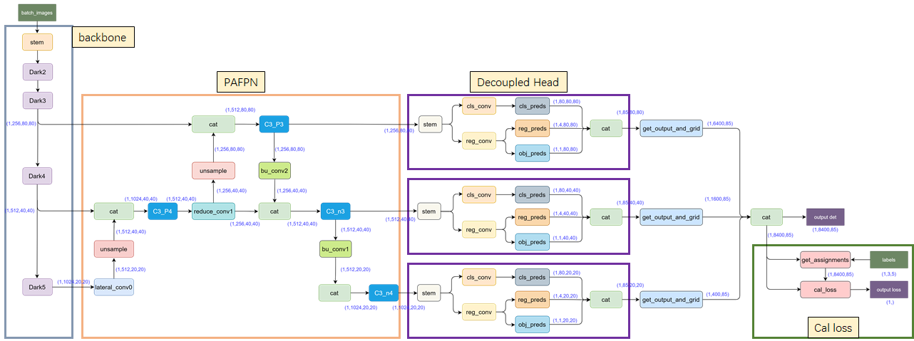
在这里插入图片描述

输入端 ：表示输入的图片，采用的数据增强方式：RandomHorizontalFlip、ColorJitter、多尺度增强
BackBone ：用来提取图片特征，采用 Darknet53。
Neck：用于特征融合，采用 PAFPN。
Head：用来结果预测，主要亮点是采用Decoupled Head、Anchor-free、Multi positives

3 YOLOX 实施细节

3.1 backbone

self.backbone = CSPDarknet(depth, width, depthwise=depthwise, act=act)

实例化backbone，采用的是 darknet53。

darknet53具体结构参考下面的图片，左侧是 darknet-53 结构图，右侧是对左侧中的 “convolutional” 层和 “residual” 层的细节展示。

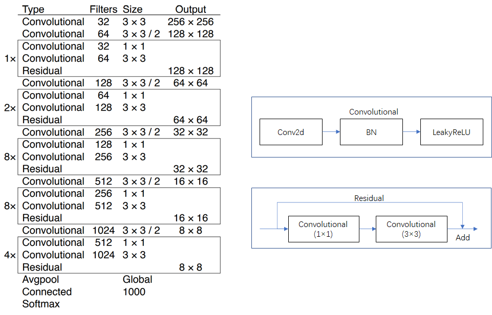
为什么使用 darknet-53 backbone？

darknet-53 的性能接近 ResNet-152，但是 FPS 要高一倍。

out_features = self.backbone(input)

backbone的输入input为一个batch的图片 (B,C,H,W)，其中B为batchsize，C为图片的channel数，如果是RGB图片，则C=3，H，W分别是图片的高宽。

假设batchsize为1，宽高分别为640,640，则 demo input可以表示为： torch.randn((1,3,640,640))。

out_features的输出为3个特征层（分别为’dark3’,‘dark4’,‘dark5’）组成的字典，各特征层的shape如下：

{'dark3':(1,256,80,80),
 'dark4':(1,512,40,40),
 'dark5':(1,1024,20,20)}

3.2 neck

features =[out_features[f]for f in self.in_features][x2, x1, x0]= features
# x0:(1,1024,20,20)# x1:(1,512,40,40)# x2:(1,256,80,80)

fpn_out0 = self.lateral_conv0(x0)# (1,512,20,20)

f_out0 = self.upsample(fpn_out0)# (1,512,40,40)
f_out0 = torch.cat([f_out0, x1],1)# (1,1024,40,40)
f_out0 = self.C3_p4(f_out0)# (1,512,40,40)

fpn_out1 = self.reduce_conv1(f_out0)# (1,256,40,40)
f_out1 = self.upsample(fpn_out1)# (1,256,80,80)
f_out1 = torch.cat([f_out1, x2],1)# (1,512,80,80)
pan_out2 = self.C3_p3(f_out1)# (1,256,80,80)

p_out1 = self.bu_conv2(pan_out2)# (1,256,40,40)
p_out1 = torch.cat([p_out1, fpn_out1],1)# (1,512,40,40)
pan_out1 = self.C3_n3(p_out1)# (1,512,40,40)

p_out0 = self.bu_conv1(pan_out1)# (1,512,20,20)
p_out0 = torch.cat([p_out0, fpn_out0],1)# (1,1024,20,20)
pan_out0 = self.C3_n4(p_out0)# (1,1024,20,20)

outputs =(pan_out2, pan_out1, pan_out0)

在Neck结构中，Yolox采用PAFPN的结构进行融合。如下图所示，将高层的特征信息，先通过上采样的方式进行传递融合，再通过下采样融合方式得到预测的特征图，最终输出3个特征层组成的元组结果，各特征层的shape如下：

((1,256,80,80),(1,512,40,40),(1,1024,20,20))

$[外链图片转存失败,源站可能有防盗链机制,建议将图片保存下来直接上传(img-2dEj8WvJ-1649596892593)(C:\Users\Sunny\AppData\Roaming\Typora\typora-user-images\image-20220410181246195.png)]$

3.3 Head

为了便于理解，我们假定图片上有3个目标框，即3个groundtruth，再假定项目有80个检测类别，则head 输出维度为85 (80+1+4)，其中80为类别分数，为1为目标分数，4为bbox的坐标。

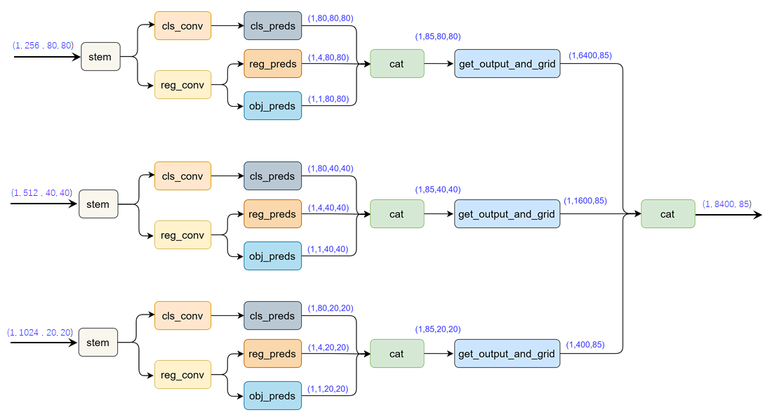
3.3.1 Decoupled Head

之前yolo 系列都是使用coupled head， yolox使用decoupled head。

coupled head 和 decoupled head 有什么差异？

当使用coupled head时，网络直接输出shape (1,85,80,80);
如果使用 decoupled head，网络会分成回归分支和分类分支，最后再汇总在一起，得到shape同样为 (1,85,80,80)。

为什么用decoupled head？

如果使用coupled head，输出channel将分类任务和回归任务放在一起，这2个任务存在冲突性。

通过实验发现替换为Decoupled Head后，不仅是模型精度上会提高，同时 网络的收敛速度也加快了，使用Decoupled Head的表达能力更好。

Yolo Head和 Decoupled Head 的对比曲线如下：

3.3.2 Anchor-free

有2种经典的anchor free目标检测模型，分别为

FCOS

和

CenterNet

，参考如下博客：

目标检测: 一文读懂 CenterNet (CVPR 2019)_大林兄的博客-CSDN博客

目标检测: 一文读懂 FCOS (CVPR 2019)_大林兄的博客-CSDN博客

如果只指定一个点作为positive，很多其他高质量的预测如果不纳入来计算loss，这不利于训练，

Yolox使用FCOS中的center sampling方法，将目标中心3x3的区域内的像素点都作为 target，这在Yolox论文中称为 multi positives。

3.4 如何计算Loss

进行Loss 计算前，需要将不同特征层的输出预测框映射回原图。通过

get_output_and_grid

函数实现，核心代码如下：

hsize, wsize = output.shape[-2:]# hsize：80, wsize：80 
yv, xv = meshgrid([torch.arange(hsize), torch.arange(wsize)])#yv, xv shape: (1,85,80,80),(1,85,80,80)
grid = torch.stack((xv, yv),2).view(1,1, hsize, wsize,2).type(dtype)#grid shape: (1,1,85,80,80)
grid = grid.view(1,-1,2)#grid shape: (1,6400,2)

output[...,:2]=(output[...,:2]+ grid)* stride  
#output shape: (1,6400,85)

output[...,2:4]= torch.exp(output[...,2:4])* stride
#output shape: (1,6400,85)

代码中前4行是生成gird的坐标，第5行则计算bbox中心坐标。

因为head关于bbox的输出位置是相对grid的距离，所以映射回原图需要加上grid坐标。

宽高尺寸为正数，所以对output的宽高先做指数运算，再乘上stride，得到原图尺度下的宽高。

最后将3个特征图上的预测框结果合并，得到所有的预测框结果，输出shape为(1,8400,85)。

得到预测结果之后，如果是推断，只要输出

output det

即可。

如果是训练，需要通过函数

get_assignments

先得到 8400个预测框的

target

，即标签分配，随后再进行

loss

计算。

如果得到了 target，loss计算公式如下：

     l
    
    
     o
    
    
     s
    
    
     s
    
    
     =
    
    
     λ
    
    
     ⋅
    
    
     l
    
    
     o
    
    
     s
    
    
     
      s
     
     
      
       r
      
      
       e
      
      
       g
      
     
    
    
     +
    
    
     l
    
    
     o
    
    
     s
    
    
     
      s
     
     
      
       o
      
      
       b
      
      
       j
      
     
    
    
     +
    
    
     l
    
    
     o
    
    
     s
    
    
     
      s
     
     
      
       c
      
      
       l
      
      
       s
      
     
    
    
     +
    
    
     l
    
    
     o
    
    
     s
    
    
     
      s
     
     
      
       l
      
      
       1
      
     
    
   
   
     loss=\lambda \cdot loss_{reg}+loss_{obj}+loss_{cls}+loss_{l1} 
   
  
 loss=λ⋅lossreg+lossobj+losscls+lossl1

代码实现如下：

loss_iou =(self.iou_loss(bbox_preds.view(-1,4)[fg_masks], reg_targets)).sum()/ num_fg
loss_obj =(self.bcewithlog_loss(obj_preds.view(-1,1), obj_targets)).sum()/ num_fg
loss_cls =(self.bcewithlog_loss(cls_preds.view(-1, self.num_classes)[fg_masks], cls_targets)).sum()/ num_fg

if self.use_l1:
    loss_l1 =(self.l1_loss(origin_preds.view(-1,4)[fg_masks], l1_targets)).sum()/ num_fg
else:
    loss_l1 =0.0

reg_weight =5.0
loss = reg_weight * loss_iou + loss_obj + loss_cls + loss_l1

3.5 如何分配标签?

经过 3个head的输出，一共有8400个预测框，这8400个预测框的标签是什么？

这8400个预测框绝大部分是负样本，只有少数是正样本，直接对8400个预测框做精确的标签分配，计算量较大。

yolox分配标签过程分为2步：(1) 粗筛选；（2）simOTA 精确分配标签

step1：粗筛选

筛选出潜在包含正样本的预测框，参见代码： get_in_boxes_info

如果

anchor bbox

中心落在

groundtruth bbox

或

fixed bbox

，则被选中为候选正样本。

<1> 判断 anchor bbox 中心是否在 groundtruth bbox

step1：计算groundtruth的左上角、右下角坐标

groundtruth的 gt_bboxes_per_image为：[x_center,y_center，w，h]。

可以根据此信息可以计算出groundtruth 的左上角、右下角坐标：

## 方法1(groundtruth bbox): l,r,t,b
gt_bboxes_per_image_l =((gt_bboxes_per_image[:,0]-0.5* gt_bboxes_per_image[:,2]).unsqueeze(1).repeat(1, total_num_anchors))# shape:(3,8400)

gt_bboxes_per_image_r =((gt_bboxes_per_image[:,0]+0.5* gt_bboxes_per_image[:,2]).unsqueeze(1).repeat(1, total_num_anchors))# shape:(3,8400)

gt_bboxes_per_image_t =((gt_bboxes_per_image[:,1]-0.5* gt_bboxes_per_image[:,3]).unsqueeze(1).repeat(1, total_num_anchors))# shape:(3,8400)

gt_bboxes_per_image_b =((gt_bboxes_per_image[:,1]+0.5* gt_bboxes_per_image[:,3]).unsqueeze(1).repeat(1, total_num_anchors))# shape:(3,8400)

step2：判断anchor bbox 中心是否落在groudtruth边框范围内

前4行代码计算锚框中心点（x_center，y_center），和人脸标注框左上角（gt_l，gt_t），右下角（gt_r，gt_b）两个角点的相应距离。

b_l = x_centers_per_image - gt_bboxes_per_image_l  # shape:(3,8400)
b_r = gt_bboxes_per_image_r - x_centers_per_image  # shape:(3,8400)
b_t = y_centers_per_image - gt_bboxes_per_image_t  # shape:(3,8400)
b_b = gt_bboxes_per_image_b - y_centers_per_image  # shape:(3,8400)

bbox_deltas = torch.stack([b_l, b_t, b_r, b_b],2)# shape:(3,8400,4)
is_in_boxes = bbox_deltas.min(dim=-1).values >0.0# shape:(3,8400)
is_in_boxes_all = is_in_boxes.sum(dim=0)>0# shape:(8400,)

第5行将四个值叠加之后，通过第六行，判断是否都大于0？ 就可以将落在groundtruth矩形范围内的所有anchors，都提取出来了。

因为ancor box的中心点，只有落在矩形范围内，这时的b_l，b_r，b_t，b_b都大于0。

<2> 判断anchor bbox 中心是否在 fixed bbox

以groundtruth的中心点为中心，在特征层尺度上做

如果图片的尺寸为

    640
   
   
    ×
   
   
    640
   
  
  
   640\times 640
  
 
640×640，且当前特征图的尺度为 

 
  
   
    80
   
   
    ×
   
   
    80
   
  
  
   80 \times 80
  
 
80×80，则此时stride为 8， 将 

 
  
   
    5
   
   
    ×
   
   
    5
   
  
  
   5 \times 5
  
 
5×5 的正方形映射回原图，fixed bbox 尺寸为 

 
  
   
    400
   
   
    ×
   
   
    400
   
  
  
   400 \times 400
  
 
400×400。

所以如果 ancor box的中心点落在 fixed bbox范围内，也将被选中。

## 方法2(fixed bbox): l,r,t,b
center_radius =2.5

gt_bboxes_per_image_l =(
    gt_bboxes_per_image[:,0]).unsqueeze(1).repeat(1, total_num_anchors
)- center_radius * expanded_strides_per_image.unsqueeze(0)

gt_bboxes_per_image_r =(
    gt_bboxes_per_image[:,0]).unsqueeze(1).repeat(1, total_num_anchors
)+ center_radius * expanded_strides_per_image.unsqueeze(0)

gt_bboxes_per_image_t =(
    gt_bboxes_per_image[:,1]).unsqueeze(1).repeat(1, total_num_anchors
)- center_radius * expanded_strides_per_image.unsqueeze(0)

gt_bboxes_per_image_b =(
    gt_bboxes_per_image[:,1]).unsqueeze(1).repeat(1, total_num_anchors
)+ center_radius * expanded_strides_per_image.unsqueeze(0)

未选中的预测框为负样本，直接打上负样本标签。

(2) step2：simOTA

经过粗筛选，假设筛选出1000个预测框为潜在正样本，这1000个预测框并不是都作为正样本分配标签，而是需要进一步做标签分配，yolox使用simOTA方法，该方法的详细介绍参见博客：

目标检测: 一文读懂 OTA 标签分配_大林兄的博客-CSDN博客

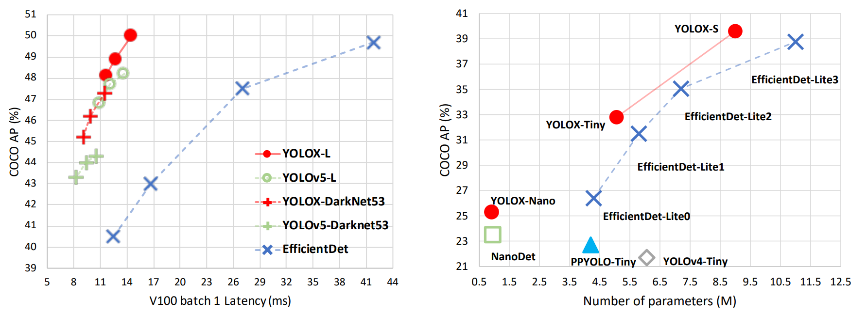
4 YOLOX 性能效果

YOLOX的性能超越了YOLOV5，YOLOX-X的AP值达到了51.2，超过YOLOV5-X 0.8个百分点，此外模型推理速度和参数量都具有比较大的优势。

$[外链图片转存失败,源站可能有防盗链机制,建议将图片保存下来直接上传(img-YRqdfXsk-1649596892595)(C:\Users\Sunny\AppData\Roaming\Typora\typora-user-images\image-20220410204605863.png)]$
在这里插入图片描述

5 总结

YOLOX做出了如下贡献：

(1) 将 anchor free 方法引入到YOLO系列，性能超越了基于anchor based方法的yolov5；

(2) 采用了 decoupled head、simOTA等方法，值得借鉴。

在这里插入图片描述

标签：计算机视觉目标检测深度学习

本文转载自: https://blog.csdn.net/weixin_46142822/article/details/124086230
版权归原作者 大林兄 所有，如有侵权，请联系我们删除。